Tianyi Zhang is a graduate student under the supervision of Professor Yongquan Xue at University of Science and Technology of China. His research is focused on active galactic nuclei
Yongquan Xue is currently a Professor at University of Science and Technology of China. He received his Ph.D. degree from Purdue University. His research interests mainly focus on active galactic nuclei and high-energy astrophysics
We present a routinized and reliable method to obtain source catalogs from the Nuclear Spectroscopic Telescope Array (NuSTAR) extragalactic surveys of the Extended Chandra Deep Field-South (E-CDF-S) and Chandra Deep Field-North (CDF-N). The NuSTAR E-CDF-S survey covers a sky area of ∼30′×30′ to a maximum depth of ∼230ks corrected for vignetting in the 3–24 keV band, with a total of 58 sources detected in our E-CDF-S catalog; the NuSTAR CDF-N survey covers a sky area of ∼7′×10′ to a maximum depth of ∼440ks corrected for vignetting in the 3–24 keV band, with a total of 42 sources detected in our CDF-N catalog that is produced for the first time. We verify the reliability of our two catalogs by crossmatching them with the relevant catalogs from the Chandra X-ray observatory and find that the fluxes of our NuSTAR sources are generally consistent with those of their Chandra counterparts. Our two catalogs are produced following the exact same method and made publicly available, thereby providing a uniform platform that facilitates further studies involving these two fields. Our source-detection method provides a systematic approach for source cataloging in other NuSTAR extragalactic surveys.
Graphical Abstract
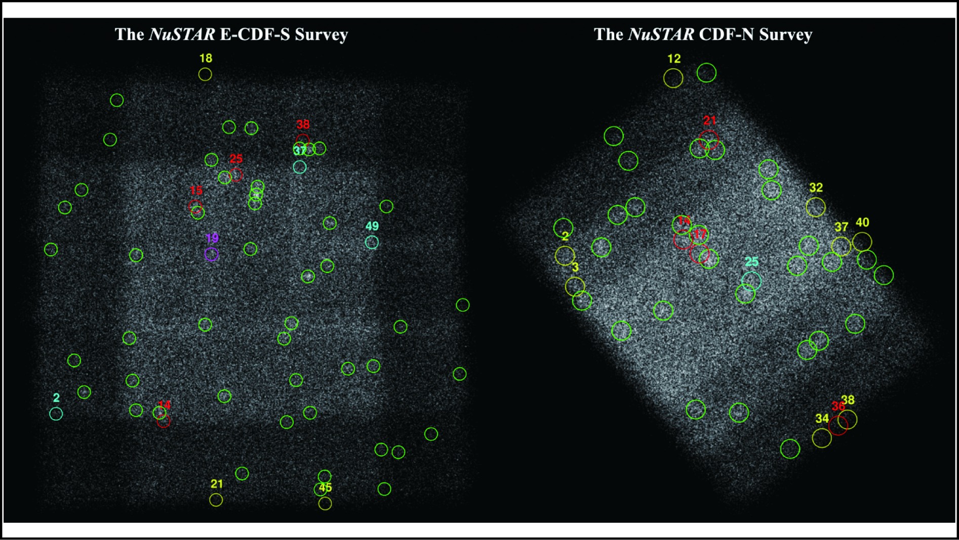
Stacked NuSTAR E-CDF-S and CDF-N science mosaics in the 3–24 keV band.
Abstract
We present a routinized and reliable method to obtain source catalogs from the Nuclear Spectroscopic Telescope Array (NuSTAR) extragalactic surveys of the Extended Chandra Deep Field-South (E-CDF-S) and Chandra Deep Field-North (CDF-N). The NuSTAR E-CDF-S survey covers a sky area of ∼30′×30′ to a maximum depth of ∼230ks corrected for vignetting in the 3–24 keV band, with a total of 58 sources detected in our E-CDF-S catalog; the NuSTAR CDF-N survey covers a sky area of ∼7′×10′ to a maximum depth of ∼440ks corrected for vignetting in the 3–24 keV band, with a total of 42 sources detected in our CDF-N catalog that is produced for the first time. We verify the reliability of our two catalogs by crossmatching them with the relevant catalogs from the Chandra X-ray observatory and find that the fluxes of our NuSTAR sources are generally consistent with those of their Chandra counterparts. Our two catalogs are produced following the exact same method and made publicly available, thereby providing a uniform platform that facilitates further studies involving these two fields. Our source-detection method provides a systematic approach for source cataloging in other NuSTAR extragalactic surveys.
Public Summary
We present a routinized and reliable method to obtain source catalogs from the nuclear spectroscopic telescope array (NuSTAR) extragalactic surveys of the Extended Chandra Deep Field-South (E-CDF-S) and Chandra Deep Field-North (CDF-N).
There are 58 and 42 sources in our NuSTAR E-CDF-S and CDF-N catalogs, respectively, with the CDF-N catalog being produced for the first time.
We make our E-CDF-S and CDF-N catalogs publicly available, thereby providing a uniform platform that facilitates further studies involving these two fields.
Extragalactic X-ray surveys are efficient at identifying and characterizing highly reliable and fairly complete samples of active galactic nuclei (AGNs), given the following reasons (see, e.g., Brandt and Hasinger[1], Brandt and Alexander[2], Xue[3], for reviews). First, X-ray emission is a nearly universal feature of luminous AGNs, which can be produced in various accretion disk (plus corona) models for AGNs (e.g., Yuan and Narayan[4]). Second, X-ray emission, especially hard X-ray emission (⩾10keV), can penetrate through materials with hydrogen column densities even up to NH∼1025cm−2, which is key to excavating the majority of the AGN family, i.e., highly obscured and even Compton-thick AGNs (e.g., Li et al.[5, 6]). Third, X-ray emission is subject to minimal dilution by host-galaxy stellar emission and is powerful for probing the immediate vicinity of supermassive black holes (SMBHs) in AGNs even at high redshifts. Last, the production of the X-ray spectrum goes through numerous line and continuum emission processes, and a high-quality X-ray spectrum is effective to infer physical conditions near the central SMBH.
X-ray surveys have resolved a very large portion (∼80%−90%) of the cosmic X-ray background (CXRB) up to ∼10keV, with AGNs being the dominant contributor (e.g., Hickox and Markevitch[7], Xue et al.[8, 9], Lehmer et al.[10], Luo et al.[11]), but the resolved fraction around the peak of the CXRB at \sim 20–40\;\text{keV} has been very low (< 10\%lt; 10\%$; see, e.g., Brandt and Hasinger[1], Brandt and Alexander[2]; Harrison et al.[12]). The Nuclear Spectroscopic Telescope Array (NuSTAR), the first focusing high-energy X-ray (3–79 keV) telescope in orbit, has largely broadened the window of X-ray observations[13]. The NuSTAR surveys have resolved ~33%–39% of the 8–24 keV CXRB[12], thereby helping us better understand the contribution of highly obscured and Compton-thick AGNs to the CXRB.
The Chandra Deep Fields (CDFs), consisting of the Chandra Deep Field-South (CDF-S, Luo et al.[11], hereafter L17), Chandra Deep Field-North (CDF-N, Xue et al.[14], hereafter X16), and Extended Chandra Deep Field-South (E-CDF-S, X16), are important sky areas for study, e.g., AGN demography, physics, and evolution[3]. The Chandra X-ray observatory has accumulated ~7 Ms exposure in the CDF-S (L17), the deepest X-ray exposure ever made, which provides a large sample of AGNs at z~0–5 for powerful statistical studies. As a parallel field to the CDF-S and being the second deepest X-ray survey, the 2 Ms CDF-N (X16) effectively complements the 7 Ms CDF-S, accounting for cosmic variance and enabling comparative studies between fields. NuSTAR has also observed the CDFs for complementary studies over 10 keV, and has completed a series of additional extragalactic hard X-ray surveys[12]. Mullaney et al.[15] (hereafter M15) has released a source catalog from the NuSTAR E-CDF-S survey; however, the NuSTAR CDF-N catalog is still absent.
In this work, we propose a uniform and reliable method to process the NuSTAR E-CDF-S and CDF-N observations and perform source detection. Referring to the previous NuSTAR E-CDF-S cataloging work (M15), we obtain both the NuSTAR E-CDF-S and CDF-N source catalogs in a routinized and unified way. We describe the production of both catalogs in Section 2 and Section 3, where, for brevity, the data reduction and source detection are introduced in detail only for the E-CDF-S. We summarize our results in Section 4. We use J2000.0 coordinates and a cosmology of H_0=71\;{{\rm{km}}\cdot {\rm{s}}^{-1}\cdot {\rm{Mp}}\cdot}c^{-1}, \varOmega_{\rm{M}}=0.27, and \varOmega_{\Lambda}=0.73.
2.
Production of the NuSTAR E-CDF-S point-source catalog
2.1
Data reduction
We collect 33 valid observations from the NuSTAR E-CDF-S survey that cover a sky area of \sim 30{'}\times 30{'}, almost each of which has an effective exposure of \sim 45\;\text{ks}. The details of these observations are presented in Table 1.
Table
1.
Details of the NuSTAR E-CDF-S observations.
Obs. ID
Obs. Name
Obs. Date
RA
DEC
t_{\rm eff}
60022001002
ECDFS_MOS001
2012-09-28
52.93
−27.97
49.0
60022002001
ECDFS_MOS002
2012-09-29
52.93
−27.97
50.3
60022003001
ECDFS_MOS003
2012-09-30
52.93
−27.97
50.2
60022004001
ECDFS_MOS004
2012-10-01
52.93
−27.97
50.9
60022005001
ECDFS_MOS005
2012-10-02
53.06
−27.86
50.5
60022006001
ECDFS_MOS006
2012-10-04
53.06
−27.86
49.2
60022007002
ECDFS_MOS007
2012-11-30
53.06
−27.86
51.7
60022008001
ECDFS_MOS008
2012-12-01
53.06
−27.86
51.7
60022009001
ECDFS_MOS009
2012-12-03
53.18
−27.75
50.3
60022010001
ECDFS_MOS010
2012-12-04
53.18
−27.75
51.2
60022011001
ECDFS_MOS011
2012-12-05
53.18
−27.75
51.7
60022012001
ECDFS_MOS012
2012-12-06
53.18
−27.75
52.1
60022013001
ECDFS_MOS013
2012-12-07
53.31
−27.64
52.5
60022014001
ECDFS_MOS014
2012-12-08
53.31
−27.64
52.9
60022015001
ECDFS_MOS015
2012-12-09
53.31
−27.64
53.2
60022016001
ECDFS_MOS016
2012-12-10
53.31
−27.64
50.1
60022016003
ECDFS_MOS016
2013-03-15
52.93
−27.64
51.7
60022015003
ECDFS_MOS015
2013-03-17
52.93
−27.64
51.2
60022014002
ECDFS_MOS014
2013-03-18
52.93
−27.64
51.4
60022013002
ECDFS_MOS013
2013-03-19
52.93
−27.64
49.7
60022012002
ECDFS_MOS012
2013-03-20
53.06
−27.75
49.7
60022011002
ECDFS_MOS011
2013-03-21
53.06
−27.75
48.9
60022010002
ECDFS_MOS010
2013-03-22
53.06
−27.75
32.5
60022010004
ECDFS_MOS010
2013-03-23
53.06
−27.75
16.4
60022009003
ECDFS_MOS009
2013-03-24
53.18
−27.75
49.5
60022008002
ECDFS_MOS008
2013-03-25
53.18
−27.86
49.8
60022007003
ECDFS_MOS007
2013-03-26
53.18
−27.86
49.6
60022006002
ECDFS_MOS006
2013-03-27
53.18
−27.86
48.7
60022005002
ECDFS_MOS005
2013-03-28
53.31
−27.86
49.3
60022004002
ECDFS_MOS004
2013-03-29
53.31
−27.97
48.8
60022003002
ECDFS_MOS003
2013-03-30
53.31
−27.97
49.0
60022002002
ECDFS_MOS002
2013-03-31
53.31
−27.97
49.0
60022001003
ECDFS_MOS001
2013-04-01
52.93
−27.97
48.2
Obs. ID is a unique identification number specifying the NuSTAR observation; Obs. Name gives the designation of the target at which NuSTAR was pointing. Obs. Date is the start time of the observation. RA and DEC give the J2000.0 Right Ascension and the Declination of the NuSTAR pointing position. t_{\rm eff} is the effective exposure time (in ks) after background filtering (see Section 2.1.1).
As NuSTAR is composed of two focal plane modules (i.e., FPMA and FPMB), each of the 33 observations results in two event files. We use the program nupipeline of the NuSTAR data analysis software NuSTARDAS to generate 66 initial event files with default parameters. Following M15, full-field lightcurves in the entire energy band (i.e., 3–78 keV) with a bin size of 20 s are produced to inspect the influence of flaring events. The dmgti tool of the Chandra interactive analysis of observations (CIAO) is used to make a user-defined good-time interval (GTI) file to avoid background flaring when the average binned count rate exceeds 1.5\;{\rm{cts}} \cdot {{\rm{s}}^{ - 1}} in the light curves. Taking the GTI files into account, we run nupipeline again to obtain the 66 cleaned event files. Following Alexander et al.[16], the final cleaned event files are split into three standard energy bands, 3–8 keV (soft band; S), 8–24 keV (hard band; H), and 3–24 keV (full band; F), respectively.
2.1.2
Science, exposure, and background mosaics
From the cleaned event files, we produce exposure maps with the NuSTARDAS program nuexpomap. For the effects of vignetting, the same energy correction values as those in M15 are adopted to generate the effective exposure maps, i.e., 5.42 keV, 13.02 keV, and 9.88 keV for the soft, hard, and full bands, respectively. The E-CDF-S reaches a maximum depth of \sim 230 \;\text{ks} corrected for vignetting in the full band.
Due to the high count-rate backgrounds in the NuSTAR E-CDF-S observations, we generate model background maps using the IDL software nuskybgd[17]. Following a similar strategy adopted by M15, we choose 4 large (i.e., radius of 3{'}) circular regions centered on the 4 chips of the detector as our background regions. With the user-defined regions, the nuskybgd software can extract and fit the corresponding spectra in XSPEC with the preset models and derive the best-fit parameters. These parameters are used to generate “fake” background images of the observations. Using the FTOOLS task XIMAGE, these simulated images are collected and merged into background mosaics weighted by the corresponding exposure maps; similarly, using XIMAGE, the stacked science mosaics (see Fig. 1) are directly produced from the cleaned event files.
Figure
1.
Stacked NuSTAR E-CDF-S science mosaic in the full band, with a total of 58 sources plotted as circles. The green (47/58) and red (4/58; being less significant detections) sources have the Chandra 250 ks E-CDF-S counterparts within r_{\rm m}=30'' . The magenta source (1/58) does not have any Chandra 250 ks E-CDF-S counterparts but can be matched to a Chandra 7 Ms CDF-S source. Among the unmatched sources (6/58), 3 yellow sources reside in the very edges of the mosaic and 3 cyan sources reside in the chip-gap areas. Numbers are source XIDs. The bottom color bar indicates the counts per pixel.
We note that in the newest version of nuskybgd, the use of the “nuabs” XSPEC model has been phased out of nuskybgd routines. However, we find that when “nuabs” is removed, the model background counts are significantly lower than what they should be. Consequently, we turn to using the old version that includes the “nuabs” model in the spectral fitting process.
2.2
Source detection
As shown in Fig. 1, traditional source detection methods (e.g., WAVDETECT[18] and ACIS Extract[19] adopted in Xue et al.[8, 14], Luo et al.[11]) are invalid due to the heavy background. Following the general strategy adopted for NuSTAR surveys (M15, Masini et al.[20]), we use the incomplete Gamma (igamma) function (see Georgakakis et al.[21]) in the Scipy.special package to produce false probability ( P_{\rm false} ) maps for source detection:
where N_{\rm Sci} and N_{\rm Bgd} represent the photon counts within one region at the same position in the science and background mosaics. The P_{\rm false} value gives the probability that a signal with N_{\rm Sci} counts is purely due to random fluctuation given the background of N_{\rm Bgd} , which means that the signal is more likely to be real as P_{\rm false} decreases.
We smooth the science and background mosaics with top-hat functions of different radii, with the former ( 10'' ) being smaller for finer structures and the latter ( 20'' ) being larger to decrease the background influence. The P_{\rm false} maps are produced using three methods: (ⅰ) the P_{\rm false} value at the position ( x , y ) is directly derived by igamma(Sci( x , y ), Bgd( x , y )), where the resulting P_{\rm false} maps are called P_{r0} maps. (ⅱ) At position ( x , y ), we perform aperture photometry with a circular region of radius 10'' on the mosaics and then calculate the P_{\rm false} value from igamma(Sci_{10''}(x,\;y), Bgd_{10''}(x,\;y)), where the resulting P_{\rm false} maps are called P_{r10} maps. (ⅲ) The same procedure as method (ⅱ) but using a 20'' radius aperture is adopted to obtain the P_{r20} maps. Considering the potential signals residing in the local minima of the P_{\rm false} maps, we produce the inverse P_{\rm false} maps using \log({1/P_{\rm false}}) to identify peaks with the SExtractor source-detection algorithm[22].
Some modifications on the default SExtractor configuration file default.sex are listed below:
(Ⅰ) DETECT_MINAREA is set to 1. Because we smooth the input maps, even one pixel in the 1/ P_{\rm false} maps can be considered as a potential source.
(Ⅱ) THRESH_TYPE is set to ABSOLUTE. Under this condition, DETECT_THRESH represents the detection threshold above which a signal in the maps can be considered significant.
(Ⅲ) FILTER and CLEAN are set to N(o). We do not need these processes as what we address here are not real observational images.
With proper DETECT_THRESH values, SExtractor is able to detect potential sources in the three standard bands to produce our initial catalogs.
2.2.1
Simulations
We perform a series of simulations to determine DETECT_THRESH. Because the science mosaics are smoothed with the 10'' -radius circular top-hat function (see Section 2.2), we split the background images into several square cells with a side length of 20'' . For every background image, Poisson realizations are performed on these cells to make up a “science” image from pure Poisson fluctuation. The aforementioned procedures are then performed on these Poisson realizations, and SExtractor should detect no sources in the corresponding inverse P_{\rm false} maps with proper thresholds.
The simulations are repeated for 100 times, in each of which we produce inverse P_{\rm false} maps with three different aperture radii (i.e., 0'' , 10'' , and 20'' ) in the three standard bands. DETECT_THRESH is set to the value above which SExtractor can find no more than N signals in these simulated maps per aperture radius per band, and R=N/100 represents the false detection rate. These thresholds are applied to the real inverse P_{\rm false} maps for source detection.
2.2.2
Final catalog production
We first set R=0.1 for loose thresholds, with which our algorithm is run on the P_{r0} , P_{r10} , and P_{r20} maps to generate three seed lists in each band. These seed lists are produced from different P_{\rm false} maps; thus, there might be multiple nearby detections belonging to the same source. To identify every unique source, we merge the seed lists for each band and then run a modified friends-of-friends algorithm (hereafter FOF) on these merged lists for deduplication.
FOF is common in cosmology for identifying groups in dense fields[23], which demands that any particle (or galaxy) that finds another one within a distance l (called linking length) should be linked to it to form a group. Sources in the merged lists are split into group sources and isolated sources by FOF with a linking length of 30'' . For each group, members are ranked by their inverse P_{r20} values (even if being initially detected from other P_{\rm false} maps), then compete against any others within a 30'' radius, in which a member of higher value can survive and participate in a next competition. After several rounds of competitions, the final survivals from the group sources are combined with the isolated sources to make up the deduplicated seed lists for each band.
The deduplicated seed lists from different bands are combined into one seed list and then split by FOF in the same way. For each group in the combined list, members are ranked by their inverse P_{r20} values in the full band (regardless of whether being detected in this band), then participate in competitions against each other. After deduplication, the remaining sources are collected to construct our seed catalog with R=0.1 . The details are presented in Table 2.
To produce a reliable final catalog, we then set R=0.01 , which means only 1 false signal being detected in 100 simulations. The thresholds of the inverse P_{r20} maps are 3.99, 4.36, and 4.33 in the soft, hard, and full bands, respectively, corresponding to \sim99\% reliability[24]. We remove the sources that do not meet any of our final thresholds and construct the final catalog with the remaining ones.
The E-CDF-S final catalog contains 58 sources, each of which is detected in at least one of the three standard bands. Of these 58 sources, 33, 13, and 54 are detected in the soft, hard, and full bands, respectively; 3, 1, and 21 are detected only in the soft, hard, and full bands, respectively; no source is detected in exactly the soft and hard bands, 21 in exactly the soft and full bands, and 3 in exactly the hard and full bands; and 9 are detected in all the three standard bands.
2.2.3
Photometry and deblending
The radius of the 90% encircled-energy fraction contour of the NuSTAR point spread function (PSF) is approximately 67.5'' , which is relatively large compared to the average distance among sources. We adopt a similar strategy to that of M15 to choose an aperture size of 30'' for photometry extraction and assume that the net counts within this aperture are only contaminated by other nearby NuSTAR-detected sources within 90'' .
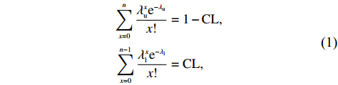
For each source in our catalog, the total and background counts are calculated within a circular region of radius 30'' in the science and background mosaics, respectively, while the net counts are derived by subtracting the background counts from the total counts. Following Gehrels[25], we estimate the upper and lower 1\sigma confidence limits on the total counts; for those not detected in certain bands, only the upper limits are derived, using:
where \lambda_{\rm{u}} and \lambda_{\rm{l}} represent the upper and lower limits, n is the photon count, and CL represents the confidence level, respectively.
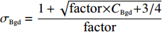
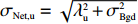
The background count error can be approximated by \sigma_{\rm Bgd}=\dfrac{1+\sqrt{\text{factor} \times C_{\rm Bgd} + 3/4}}{\text{factor}}, where C_{\rm Bgd} is the background count and the \text{factor} gives the ratio between the total area where the background model is defined and the area for photometry extraction (i.e., \text{factor}=(180''/30'')^2\times 4=144). Subsequently, the upper and lower limits on the net counts are calculated as \sigma_{\rm Net,u}=\sqrt{\lambda_{\rm{u}}^2+\sigma_{\rm Bgd}^2} and \sigma_{\rm Net,l}=\sqrt{\lambda_{\rm{l}}^2+\sigma_{\rm Bgd}^2}, respectively.
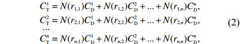
To deblend the sources in our catalog, the FOF algorithm is applied again to split them into group sources and isolated sources with a different linking length of 90'' . For the isolated sources, we assume that they cannot be contaminated by any other sources (away beyond 90'' ); for the group sources, a system of n linear simultaneous equations is established:
where C_{\rm{T}}^n is the total net counts of source n , C_{\rm{D}}^n is the deblended net counts of source n , and N(r_{i,j}) is the normalized function of the separation between the sources i and j ( r_{i,j} represents the separation distance, while N(0)=1 ), in which several simplifications are proposed to avoid the complications of the nonazimuthally symmetric NuSTAR PSF.
Following the deblending procedure above, we then perform deblending with another aperture of 20'' radius, and recalculate the P_{\rm false} of each source after deblending. The postdeblending P_{\rm false} values are compared with the P_{r20} thresholds, and 4 of the 58 sources in our catalog become no longer significant. Additionaly, we find 1 source in the area of relatively low exposure ( <40 ks, corresponding to \lesssim10\% of the maximum survey exposure). All of these 5 sources are detected in the full band only, and we flag but do not remove them (see Fig. 1).
To validate the reliability of our catalog (a total of 58 sources), we match it to the previous NuSTAR E-CDF-S catalog (a total of 54 sources) in M15 using a matching radius r_{\rm m}=30'' and find a total of 36 counterpart pairs. We compare their net counts in Fig. 2 and find good consistency within 1\sigma errors. We also compare their aperture-corrected fluxes (see Section 2.3) and find good agreement between each other.
Figure
2.
Comparison of net counts obtained by this work and M15 in the E-CDF-S. The diagonal dashed lines indicate the 1∶1 relations.
A significant fraction of the M15 sources are not detected by our work (and vice versa), mainly due to two facts: the detailed cataloging methodologies are different between our work and M15, and those unmatched sources generally have lower net counts such that they could be too faint to be detected by either work.
2.3
Matching to the Chandra E-CDF-S and CDF-S catalogs
We first match our catalog to the Chandra 250 ks E-CDF-S catalog (X16) using r_{\rm m}=30'' , and find 51 of the 58 sources to have at least one Chandra counterpart. In these matches, 20, 24, 5, and 2 NuSTAR sources have 1, 2, 3, and 4 Chandra counterparts, respectively; no NuSTAR sources has more than 4 Chandra counterparts. For the flagged sources (see Section 2.2.3), all of the 4 less-significant sources (XIDs =14, 15, 25, 38; see Fig. 1) have Chandra counterparts, but the source with low exposure time (XID = 18) does not. We then match the 7 sources without Chandra 250 ks counterparts to the Chandra 7 Ms CDF-S catalog (L17) using r_{\rm m}=30'' , only finding one further match (XID = 19).
We inspect the positions and properties of the 6 unmatched sources, finding that 3 reside in the very edge of the NuSTAR E-CDF-S survey mosaic (XIDs=18, 21, and 45; see Fig.1), which implies uncertainty in their detections. For the 3 remaining sources, one (XID = 2) is also near the edge of the mosaic and detected only in the 3–24 keV band, and the other two sources (XIDs = 37, 49) reside in the chip-gap areas (see Fig. 1) which might be spurious. Because we aim to find as many sources as possible using our algorithm alone (without manual intervention), these 6 sources are conserved and flagged in our final catalog.
To compare the fluxes of these matched sources, the observed deblended fluxes of the NuSTAR sources are derived following the same approach as Alexander et al.[16] For the sources detected in both the soft and hard bands, we calculate their hardness ratios, HR=(H−S)/(H+S), using the Bayesian estimation of hardness ratios method[26]; for other sources, an HR value corresponding to the power-law spectral photon index of \varGamma=1.8 is assumed. Using the derived HRs, the same parameters as in M15 are then adopted to convert count rates to observed fluxes (see Section 2.3.3 of M15), which reach a soft-band flux limit of \sim {10^{ - 14}}{\rm{erg}}\cdot{{\rm{s}}^{ - 1}}\cdot{\rm{c}}{{\rm{m}}^{ - 2}}.
Due to the different observable energy range of Chandra (0.5–7 keV), we assume the Chandra counterparts having a simple power-law spectrum (i.e., f(E)\propto E^{-\varGamma}), then derive the conversion factor between the fluxes in the 2–7 keV and 3–8 keV bands. The fluxes in the 2–7 keV band and photon indices (\varGamma) can be obtained from the Chandra catalogs (X16; L17). For the multiple Chandra counterparts within r_{\rm m}=30'' of the NuSTAR sources, we calculate their total 3–8 keV fluxes instead. The comparison between the NuSTAR and total Chandra 3–8 keV fluxes of the matched sources is shown in Fig. 3, which indicates general agreement within a factor of 3 for the majority of the sources. However, the NuSTAR fluxes appear to be systematically lower than the Chandra fluxes, which is mainly due to that the NuSTAR measured/assumed photon index may be different from the Chandra measured/assumed photon index (in the case of 1-to-1 match) or photon indexes (in the case of 1-to-multiple match).
Figure
3.
Comparison between the NuSTAR E-CDF-S deblended fluxes (this work) and the total Chandra E-CDF-S (X16; left panel) and CDF-S (L17; right panel) fluxes in the 3–8 keV band (all fluxes are aperture-corrected). In each panel, the green 1∶1 line is centered at the shaded area indicating a factor of \le 3 difference from the 1∶1 line, and the horizontal dotted line indicates the detection limit.
3.
Production of the NuSTAR CDF-N point-source catalog
3.1
Data reduction and source detection
We collect 12 valid observations from the NuSTAR CDF-N survey that cover a sky area of \sim 7'\times10', almost each of which has an effective exposure of \sim 50 \;\text{ks}. We summarize the information of these observations in Table 3. For data reduction, we apply the exactly same procedures as in Section 2.1, therefore the technical details are introduced briefly in this section.
Table
3.
Details of the NuSTAR CDF-N observations.
Full-field lightcurves in the entire energy band with a bin size of 20 s are produced to inspect the influence of flaring events, and a threshhold of 1.3\;{\rm{cts}}\cdot{\rm{s^{-1}}} is selected to reject the periods with high background flares. Following the same procedures in Section 2.1.2, the science, exposure, and background mosaics are created from the cleaned event files. The CDF-N reaches a maximum depth of ~440 ks corrected for vignetting in the full band, almost doubling that of the E-CDF-S. We present the stacked science mosaic in the full band in Fig. 4.
Figure
4.
Stacked NuSTAR CDF-N science mosaic in the 3–24 keV band (cf. Fig. 1), with a total of 42 sources plotted. The green (29/42) and red (4/42; being less significant detections) sources have the Chandra 2 Ms CDF-N counterparts within r_{\rm m}=30'' . Among the unmatched sources (9/42), 8 yellow sources reside in or near the edges of the mosaic, and 1 cyan source is only detected in the 8–24 keV band.
Again we set R=0.1 to obtain the seed list from the P_{\rm fasle} maps, then refilter these seed sources with a strict threshold of R=0.01 for the final catalog that contains 42 CDF-N sources, each of which is detected in at least one of the three standard bands. Of the 42 sources, 26, 11, and 31 are detected in the soft, hard, and full bands, respectively; 9, 2, and 12 are detected in the soft, hard, and full bands only, respectively; no source is detected in exactly both the soft and hard bands, 10 in exactly both the soft and full bands, and 2 in exactly both the hard and full bands; 7 are detected in all the three standard bands. After deblending, 6 of the 42 sources are no longer significant, and we still flag and keep them in our final catalog. These results are listed in Table 4.
We match our catalog to the Chandra 2 Ms CDF-N catalog (X16) using r_{\rm m}=30'' , and find 33 of the 42 sources to have at least one Chandra counterpart. In these matches, 14, 11, 4, and 3 NuSTAR sources have 1, 2, 3, and 4 Chandra counterparts, respectively, and 1 NuSTAR source has more than 4 Chandra counterparts.
For the NuSTAR sources without Chandra counterparts, we inspect their positions and properties and find that almost all of them (8/9; XIDs = 2, 3, 12, 32, 34, 37, 38, 40) reside in or near the edges of the NuSTAR CDF-N field and the remaining one (XID = 25) is only detected in the hard band which might be too “hard” to be detected by Chandra (see Fig. 4).
We compare the fluxes of these matched sources in Fig. 5, which also indicates general agreement within a factor of 3 for the majority of the sources. The normalized flux histograms of the NuSTAR CDF-N and E-CDF-S sources are compared in Fig. 6: CDF-N sources generally have lower fluxes than E-CDF-S sources, being consistent with the fact that the average NuSTAR CDF-N exposure depth (reaching a soft-band flux limit of \sim 5\times 10^{-15}\;\text{erg}\cdot \text{s}^{−1}\cdot \text{cm}^{−2}) is almost twice that of the E-CDF-S.
Figure
5.
Same as Fig. 3, but for the comparison between the NuSTAR CDF-N deblended fluxes (this work) and the total Chandra CDF-N fluxes (X16) in the 3–8 keV band (all fluxes are aperture-corrected).
In this work, we collect the original observations from the NuSTAR E-CDF-S and CDF-N surveys and produce cleaned event files. Simulated background mosaics are generated using the IDL software nuskybgd, and then processed along with science mosaics to produce P_{\rm false} maps for source detection.
For the NuSTAR E-CDF-S survey, the main results are as follows:
(Ⅰ) The E-CDF-S catalog consists of 58 sources that are detected using our algorithm without manual intervention, with 4 of them being not significant after deblending.
(Ⅱ) We compare our catalog with the previous NuSTAR E-CDF-S catalog (M15) using r_{\rm m}=30'' and find a total of 36 matches, the net counts of which agree well within 1\sigma errors.
(Ⅲ) We compare our catalog with the Chandra E-CDF-S and CDF-S catalogs (X16 and L17), and find a total of 51 matches, the fluxes of which agree well above the detection limit. All of the 4 sources being not significant after deblending have counterparts in the Chandra catalogs; and the 7 unmatched sources are flagged as being spurious but still conserved in the catalog.
For the NuSTAR CDF-N survey, the main results are as follows:
(Ⅰ) The CDF-N catalog, produced for the first time by this work, consists of 42 sources that are detected using our algorithm without manual intervention, with 6 of them being not significant after deblending.
(Ⅱ) We compare our catalog with the Chandra CDF-N catalog (X16), and find a total of 33 matches, the fluxes of which agree well above the detection limit. We flag the 9 unmatched sources as being spurious but conserve them in the catalog.
(Ⅲ) The flux limits are significantly lower in the NuSTAR CDF-N field (having deeper exposures) than that in the NuSTAR E-CDF-S field.
Our source-detection method provides a systematic approach for source cataloging in other NuSTAR extragalactic surveys. We make our NuSTAR E-CDF-S and CDF-N source catalogs publicly available (see Appendix for catalog description), which provide a uniform platform that facilitates further studies involving these two fields.
Acknowledgements
We thank the reviewers for helpful comments that improved this work. This work was supported by the National Natural Science Foundation of China (12025303, 11890693), the National Key R&D Program of China (2022YFF0503401), the K. C. Wong Education Foundation, and the China Manned Space Project (CMS-CSST-2021-A06).
Conflict of interest
The authors declare that they have no conflict of interest.
We present a routinized and reliable method to obtain source catalogs from the nuclear spectroscopic telescope array (NuSTAR) extragalactic surveys of the Extended Chandra Deep Field-South (E-CDF-S) and Chandra Deep Field-North (CDF-N).
There are 58 and 42 sources in our NuSTAR E-CDF-S and CDF-N catalogs, respectively, with the CDF-N catalog being produced for the first time.
We make our E-CDF-S and CDF-N catalogs publicly available, thereby providing a uniform platform that facilitates further studies involving these two fields.
Brandt W N, Hasinger G. Deep extragalactic X-ray surveys. Annual Review of Astronomy and Astrophysics,2005, 43: 827–859. DOI: 10.1146/annurev.astro.43.051804.102213
[2]
Brandt W N, Alexander D M. Cosmic X-ray surveys of distant active galaxies. The Astronomy and Astrophysics Review,2015, 23: 1. DOI: 10.1007/s00159-014-0081-z
[3]
Xue Y Q. The Chandra Deep Fields: Lifting the veil on distant active galactic nuclei and X-ray emitting galaxies. New Astronomy Reviews,2017, 79: 59–84. DOI: 10.1016/j.newar.2017.09.002
[4]
Yuan F, Narayan R. Hot accretion flows around black holes. Annual Review of Astronomy and Astrophysics,2014, 52: 529–588. DOI: 10.1146/annurev-astro-082812-141003
[5]
Li J, Xue Y, Sun M, et al. Piercing through highly obscured and Compton-thick AGNs in the Chandra Deep Fields. I. X-ray spectral and long-term variability analyses. The Astrophysical Journal,2019, 877: 5. DOI: 10.3847/1538-4357/ab184b
[6]
Li J, Xue Y, Sun M, et al. Piercing through highly obscured and Compton-thick AGNs in the Chandra Deep Fields. II. are highly obscured AGNs the missing link in the merger-triggered AGN-galaxy coevolution models. The Astrophysical Journal,2020, 903: 49. DOI: 10.3847/1538-4357/abb6e7
[7]
Hickox R C, Markevitch M. Absolute measurement of the unresolved cosmic X-ray background in the 0.5–8 keV band with Chandra. The Astrophysical Journal,2006, 645: 95. DOI: 10.1086/504070
[8]
Xue Y Q, Luo B, Brandt W N, et al. The Chandra Deep Field-South survey: 4 Ms source catalogs. The Astrophysical Journal Supplement Series,2011, 195: 10. DOI: 10.1088/0067-0049/195/1/10
[9]
Xue Y Q, Wang S X, Brandt W N, et al. Tracking down the source population responsible for the unresolved cosmic 6–8 keV background. The Astrophysical Journal,2012, 758: 129. DOI: 10.1088/0004-637X/758/2/129
[10]
Lehmer B D, Xue Y Q, Brandt W N, et al. The 4 Ms Chandra Deep Field-South number counts apportioned by source class: Pervasive active galactic nuclei and the ascent of normal galaxies. The Astrophysical Journal,2012, 752: 46. DOI: 10.1088/0004-637X/752/1/46
[11]
Luo B, Brandt W N, Xue Y Q, et al. The Chandra Deep Field-South survey: 7 Ms source catalogs. The Astrophysical Journal Supplement Series,2017, 228 (1): 2. DOI: 10.3847/1538-4365/228/1/2
[12]
Harrison F A, Aird J, Civano F, et al. The NuSTAR extragalactic surveys: The number counts of active galactic nuclei and the resolved fraction of the cosmic X-ray background. The Astrophysical Journal,2016, 831: 185. DOI: 10.3847/0004-637X/831/2/185
[13]
Harrison F A, Craig W W, Finn E. Christensen F E, et al. The Nuclear Spectroscopic Telescope Array (NuSTAR) high-energy X-ray mission. The Astrophysical Journal,2013, 770–637X/770/2/103. DOI: 10.1088/0004-637x/770/2/103
[14]
Xue Y Q, Luo B, Brandt W N, et al. The 2 Ms Chandra Deep Field-North survey and the 250 ks extended Chandra Deep Field-South survey: Improved point-source catalogs. The Astrophysical Journal Supplement Series,2016, 224: 15. DOI: 10.3847/0067-0049/224/2/15
[15]
Mullaney J R, Del-Moro A, Aird J, et al. The NuSTAR extragalactic surveys: Initial results and catalog from the Extended Chandra Deep Field South. The Astrophysical Journal,2015, 808: 184. DOI: 10.1088/0004-637X/808/2/184
[16]
Alexander D M, Stern D, Del Moro A, et al. The NuSTAR extragalactic survey: A first sensitive look at the high-energy cosmic X-ray background population. The Astrophysical Journal,2013, 773: 125. DOI: 10.1088/0004-637X/773/2/125
[17]
Wik D R, Hornstrup A, Molendi S, et al. NuSTAR observations of the bullet cluster: Constraints on inverse Compton emission. The Astrophysical Journal,2014, 792: 48. DOI: 10.1088/0004-637X/792/1/48
[18]
Freeman P E, Kashyap V, Rosner R, et al. A wavelet-based algorithm for the spatial analysis of Poisson data. The Astrophysical Journal Supplement Series,2002, 138: 185. DOI: 10.1086/324017
[19]
Broos P S, Townsley L K, Feigelson E D, et al. Innovations in the analysis of Chandra-ACIS observations. The Astrophysical Journal,2010, 714: 1582. DOI: 10.1088/0004-637X/714/2/1582
[20]
Masini A, Civano F, Comastri A, et al. The NuSTAR extragalactic surveys: Source catalog and the Compton-thick fraction in the UDS field. The Astrophysical Journal Supplement Series,2018, 235 (1)–4365/aaa83d. DOI: 10.3847/1538-4365/aaa83d
[21]
Georgakakis A, Nandra K, Laird E S, et al. A new method for determining the sensitivity of X-ray imaging observations and the X-ray number counts. Monthly Notices of the Royal Astronomical Society,2008, 388: 1205–1213. DOI: 10.1111/j.1365-2966.2008.13423.x
[22]
Bertin E, Arnouts S. SExtractor: Software for source extraction. Astronomy and Astrophysics Supplement Series,1996, 117: 393–404. DOI: 10.1051/aas:1996164
[23]
Y, Feng, Modi C. A fast algorithm for identifying friends-of-friends halos. Astronomy and Computing,2017, 20: 44–51. DOI: 10.1016/j.ascom.2017.05.004
[24]
Civano F, Hickox R C, Puccetti S, et al. The NuSTAR extragalactic surveys: Overview and catalog from the cosmos field. The Astrophysical Journal,2015, 808: 185. DOI: 10.1088/0004-637X/808/2/185
[25]
Gehrels N. Confidence limits for small numbers of events in astrophysical data. The Astrophysical Journal,1986, 303: 336–346. DOI: 10.1086/164079
[26]
Park T, Kashyap V L, Siemiginowska A, et al. Bayesian estimation of hardness ratios: Modeling and computations. The Astrophysical Journal,2006, 652: 610. DOI: 10.1086/507406
Figure
1.
Stacked NuSTAR E-CDF-S science mosaic in the full band, with a total of 58 sources plotted as circles. The green (47/58) and red (4/58; being less significant detections) sources have the Chandra 250 ks E-CDF-S counterparts within r_{\rm m}=30'' . The magenta source (1/58) does not have any Chandra 250 ks E-CDF-S counterparts but can be matched to a Chandra 7 Ms CDF-S source. Among the unmatched sources (6/58), 3 yellow sources reside in the very edges of the mosaic and 3 cyan sources reside in the chip-gap areas. Numbers are source XIDs. The bottom color bar indicates the counts per pixel.
Figure
2.
Comparison of net counts obtained by this work and M15 in the E-CDF-S. The diagonal dashed lines indicate the 1∶1 relations.
Figure
3.
Comparison between the NuSTAR E-CDF-S deblended fluxes (this work) and the total Chandra E-CDF-S (X16; left panel) and CDF-S (L17; right panel) fluxes in the 3–8 keV band (all fluxes are aperture-corrected). In each panel, the green 1∶1 line is centered at the shaded area indicating a factor of \le 3 difference from the 1∶1 line, and the horizontal dotted line indicates the detection limit.
Figure
4.
Stacked NuSTAR CDF-N science mosaic in the 3–24 keV band (cf. Fig. 1), with a total of 42 sources plotted. The green (29/42) and red (4/42; being less significant detections) sources have the Chandra 2 Ms CDF-N counterparts within r_{\rm m}=30'' . Among the unmatched sources (9/42), 8 yellow sources reside in or near the edges of the mosaic, and 1 cyan source is only detected in the 8–24 keV band.
Figure
5.
Same as Fig. 3, but for the comparison between the NuSTAR CDF-N deblended fluxes (this work) and the total Chandra CDF-N fluxes (X16) in the 3–8 keV band (all fluxes are aperture-corrected).
Figure
6.
Normalized distributions of deblended NuSTAR fluxes in the CDF-N and E-CDF-S.
References
[1]
Brandt W N, Hasinger G. Deep extragalactic X-ray surveys. Annual Review of Astronomy and Astrophysics,2005, 43: 827–859. DOI: 10.1146/annurev.astro.43.051804.102213
[2]
Brandt W N, Alexander D M. Cosmic X-ray surveys of distant active galaxies. The Astronomy and Astrophysics Review,2015, 23: 1. DOI: 10.1007/s00159-014-0081-z
[3]
Xue Y Q. The Chandra Deep Fields: Lifting the veil on distant active galactic nuclei and X-ray emitting galaxies. New Astronomy Reviews,2017, 79: 59–84. DOI: 10.1016/j.newar.2017.09.002
[4]
Yuan F, Narayan R. Hot accretion flows around black holes. Annual Review of Astronomy and Astrophysics,2014, 52: 529–588. DOI: 10.1146/annurev-astro-082812-141003
[5]
Li J, Xue Y, Sun M, et al. Piercing through highly obscured and Compton-thick AGNs in the Chandra Deep Fields. I. X-ray spectral and long-term variability analyses. The Astrophysical Journal,2019, 877: 5. DOI: 10.3847/1538-4357/ab184b
[6]
Li J, Xue Y, Sun M, et al. Piercing through highly obscured and Compton-thick AGNs in the Chandra Deep Fields. II. are highly obscured AGNs the missing link in the merger-triggered AGN-galaxy coevolution models. The Astrophysical Journal,2020, 903: 49. DOI: 10.3847/1538-4357/abb6e7
[7]
Hickox R C, Markevitch M. Absolute measurement of the unresolved cosmic X-ray background in the 0.5–8 keV band with Chandra. The Astrophysical Journal,2006, 645: 95. DOI: 10.1086/504070
[8]
Xue Y Q, Luo B, Brandt W N, et al. The Chandra Deep Field-South survey: 4 Ms source catalogs. The Astrophysical Journal Supplement Series,2011, 195: 10. DOI: 10.1088/0067-0049/195/1/10
[9]
Xue Y Q, Wang S X, Brandt W N, et al. Tracking down the source population responsible for the unresolved cosmic 6–8 keV background. The Astrophysical Journal,2012, 758: 129. DOI: 10.1088/0004-637X/758/2/129
[10]
Lehmer B D, Xue Y Q, Brandt W N, et al. The 4 Ms Chandra Deep Field-South number counts apportioned by source class: Pervasive active galactic nuclei and the ascent of normal galaxies. The Astrophysical Journal,2012, 752: 46. DOI: 10.1088/0004-637X/752/1/46
[11]
Luo B, Brandt W N, Xue Y Q, et al. The Chandra Deep Field-South survey: 7 Ms source catalogs. The Astrophysical Journal Supplement Series,2017, 228 (1): 2. DOI: 10.3847/1538-4365/228/1/2
[12]
Harrison F A, Aird J, Civano F, et al. The NuSTAR extragalactic surveys: The number counts of active galactic nuclei and the resolved fraction of the cosmic X-ray background. The Astrophysical Journal,2016, 831: 185. DOI: 10.3847/0004-637X/831/2/185
[13]
Harrison F A, Craig W W, Finn E. Christensen F E, et al. The Nuclear Spectroscopic Telescope Array (NuSTAR) high-energy X-ray mission. The Astrophysical Journal,2013, 770–637X/770/2/103. DOI: 10.1088/0004-637x/770/2/103
[14]
Xue Y Q, Luo B, Brandt W N, et al. The 2 Ms Chandra Deep Field-North survey and the 250 ks extended Chandra Deep Field-South survey: Improved point-source catalogs. The Astrophysical Journal Supplement Series,2016, 224: 15. DOI: 10.3847/0067-0049/224/2/15
[15]
Mullaney J R, Del-Moro A, Aird J, et al. The NuSTAR extragalactic surveys: Initial results and catalog from the Extended Chandra Deep Field South. The Astrophysical Journal,2015, 808: 184. DOI: 10.1088/0004-637X/808/2/184
[16]
Alexander D M, Stern D, Del Moro A, et al. The NuSTAR extragalactic survey: A first sensitive look at the high-energy cosmic X-ray background population. The Astrophysical Journal,2013, 773: 125. DOI: 10.1088/0004-637X/773/2/125
[17]
Wik D R, Hornstrup A, Molendi S, et al. NuSTAR observations of the bullet cluster: Constraints on inverse Compton emission. The Astrophysical Journal,2014, 792: 48. DOI: 10.1088/0004-637X/792/1/48
[18]
Freeman P E, Kashyap V, Rosner R, et al. A wavelet-based algorithm for the spatial analysis of Poisson data. The Astrophysical Journal Supplement Series,2002, 138: 185. DOI: 10.1086/324017
[19]
Broos P S, Townsley L K, Feigelson E D, et al. Innovations in the analysis of Chandra-ACIS observations. The Astrophysical Journal,2010, 714: 1582. DOI: 10.1088/0004-637X/714/2/1582
[20]
Masini A, Civano F, Comastri A, et al. The NuSTAR extragalactic surveys: Source catalog and the Compton-thick fraction in the UDS field. The Astrophysical Journal Supplement Series,2018, 235 (1)–4365/aaa83d. DOI: 10.3847/1538-4365/aaa83d
[21]
Georgakakis A, Nandra K, Laird E S, et al. A new method for determining the sensitivity of X-ray imaging observations and the X-ray number counts. Monthly Notices of the Royal Astronomical Society,2008, 388: 1205–1213. DOI: 10.1111/j.1365-2966.2008.13423.x
[22]
Bertin E, Arnouts S. SExtractor: Software for source extraction. Astronomy and Astrophysics Supplement Series,1996, 117: 393–404. DOI: 10.1051/aas:1996164
[23]
Y, Feng, Modi C. A fast algorithm for identifying friends-of-friends halos. Astronomy and Computing,2017, 20: 44–51. DOI: 10.1016/j.ascom.2017.05.004
[24]
Civano F, Hickox R C, Puccetti S, et al. The NuSTAR extragalactic surveys: Overview and catalog from the cosmos field. The Astrophysical Journal,2015, 808: 185. DOI: 10.1088/0004-637X/808/2/185
[25]
Gehrels N. Confidence limits for small numbers of events in astrophysical data. The Astrophysical Journal,1986, 303: 336–346. DOI: 10.1086/164079
[26]
Park T, Kashyap V L, Siemiginowska A, et al. Bayesian estimation of hardness ratios: Modeling and computations. The Astrophysical Journal,2006, 652: 610. DOI: 10.1086/507406
Table
1.
Details of the NuSTAR E-CDF-S observations.
Obs. ID
Obs. Name
Obs. Date
RA
DEC
t_{\rm eff}
60022001002
ECDFS_MOS001
2012-09-28
52.93
−27.97
49.0
60022002001
ECDFS_MOS002
2012-09-29
52.93
−27.97
50.3
60022003001
ECDFS_MOS003
2012-09-30
52.93
−27.97
50.2
60022004001
ECDFS_MOS004
2012-10-01
52.93
−27.97
50.9
60022005001
ECDFS_MOS005
2012-10-02
53.06
−27.86
50.5
60022006001
ECDFS_MOS006
2012-10-04
53.06
−27.86
49.2
60022007002
ECDFS_MOS007
2012-11-30
53.06
−27.86
51.7
60022008001
ECDFS_MOS008
2012-12-01
53.06
−27.86
51.7
60022009001
ECDFS_MOS009
2012-12-03
53.18
−27.75
50.3
60022010001
ECDFS_MOS010
2012-12-04
53.18
−27.75
51.2
60022011001
ECDFS_MOS011
2012-12-05
53.18
−27.75
51.7
60022012001
ECDFS_MOS012
2012-12-06
53.18
−27.75
52.1
60022013001
ECDFS_MOS013
2012-12-07
53.31
−27.64
52.5
60022014001
ECDFS_MOS014
2012-12-08
53.31
−27.64
52.9
60022015001
ECDFS_MOS015
2012-12-09
53.31
−27.64
53.2
60022016001
ECDFS_MOS016
2012-12-10
53.31
−27.64
50.1
60022016003
ECDFS_MOS016
2013-03-15
52.93
−27.64
51.7
60022015003
ECDFS_MOS015
2013-03-17
52.93
−27.64
51.2
60022014002
ECDFS_MOS014
2013-03-18
52.93
−27.64
51.4
60022013002
ECDFS_MOS013
2013-03-19
52.93
−27.64
49.7
60022012002
ECDFS_MOS012
2013-03-20
53.06
−27.75
49.7
60022011002
ECDFS_MOS011
2013-03-21
53.06
−27.75
48.9
60022010002
ECDFS_MOS010
2013-03-22
53.06
−27.75
32.5
60022010004
ECDFS_MOS010
2013-03-23
53.06
−27.75
16.4
60022009003
ECDFS_MOS009
2013-03-24
53.18
−27.75
49.5
60022008002
ECDFS_MOS008
2013-03-25
53.18
−27.86
49.8
60022007003
ECDFS_MOS007
2013-03-26
53.18
−27.86
49.6
60022006002
ECDFS_MOS006
2013-03-27
53.18
−27.86
48.7
60022005002
ECDFS_MOS005
2013-03-28
53.31
−27.86
49.3
60022004002
ECDFS_MOS004
2013-03-29
53.31
−27.97
48.8
60022003002
ECDFS_MOS003
2013-03-30
53.31
−27.97
49.0
60022002002
ECDFS_MOS002
2013-03-31
53.31
−27.97
49.0
60022001003
ECDFS_MOS001
2013-04-01
52.93
−27.97
48.2
Obs. ID is a unique identification number specifying the NuSTAR observation; Obs. Name gives the designation of the target at which NuSTAR was pointing. Obs. Date is the start time of the observation. RA and DEC give the J2000.0 Right Ascension and the Declination of the NuSTAR pointing position. t_{\rm eff} is the effective exposure time (in ks) after background filtering (see Section 2.1.1).


 DownLoad: