ISSN 0253-2778
CN 34-1054/N
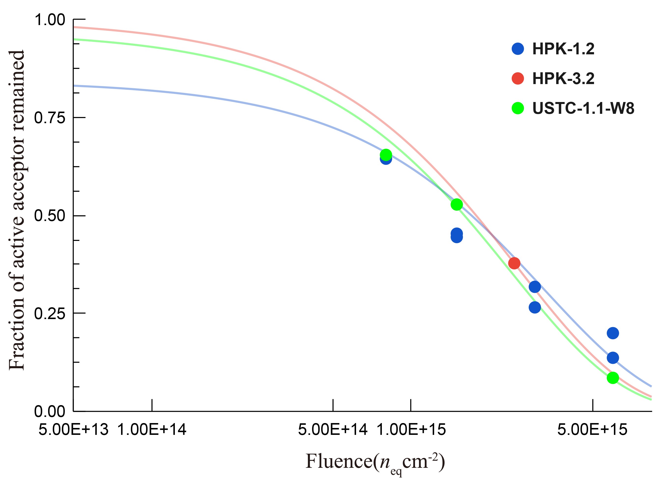
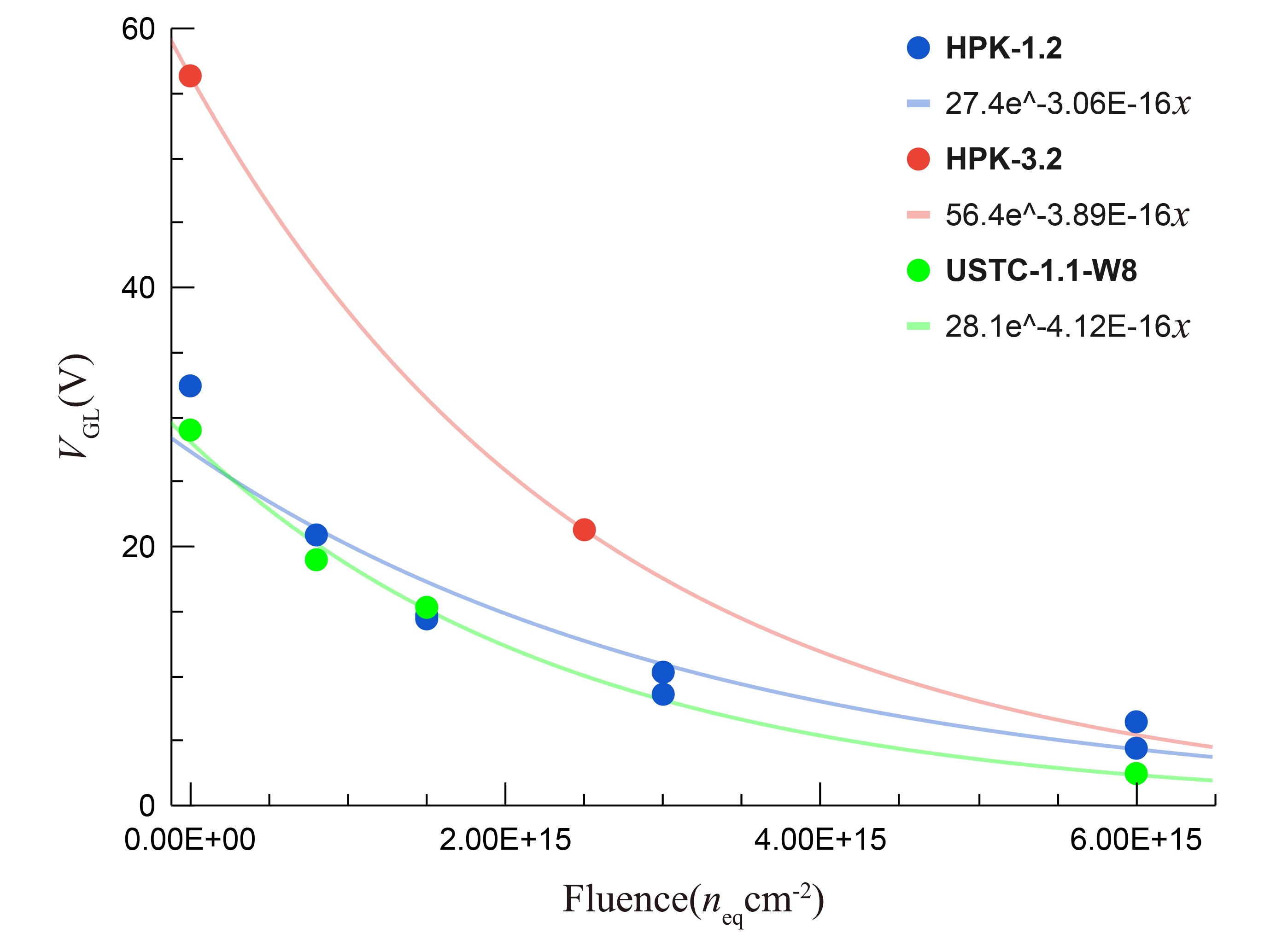
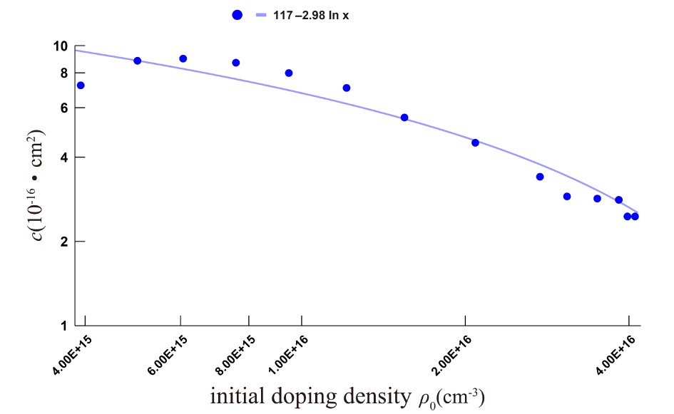
The high granularity timing detector (HGTD) is a crucial component of the ATLAS phase II upgrade to cope with the extremely high pile-up (the average number of interactions per bunch crossing can be as high as 200). With the precise timing information (σt~30 ps) of the tracks, the track-to-vertex association can be performed in the “4-D” space. The Low Gain Avalanche Detector (LGAD) technology is chosen for the sensors, which can provide the required timing resolution and good signal-to-noise ratio. Hamamatsu Photonics K.K. (HPK) has produced the LGAD with thicknesses of 35 μm and 50 μm. The University of Science and Technology of China(USTC) has also developed and produced 50 μm LGADs prototypes with the Institute of Microelectronics (IME) of Chinese Academy of Sciences. To evaluate the irradiation hardness, the sensors are irradiated with the neutron at the JSI reactor facility and tested at USTC. The irradiation effects on both the gain layer and the bulk are characterized by I-V and C-V measurements at room temperature (20 ℃) or −30 ℃. The breakdown voltages and depletion voltages are extracted and presented as a function of the fluences. The final fitting of the acceptor removal model yielded the c-factor of 3.06×10⁻¹⁶ cm−2, 3.89×10⁻¹⁶ cm−2 and 4.12×10⁻¹⁶ cm−2 for the HPK-1.2, HPK-3.2 and USTC-1.1-W8, respectively, showing that the HPK-1.2 sensors have the most irradiation resistant gain layer. A novel analysis method is used to further exploit the data to get the relationship between the c-factor and initial doping density.
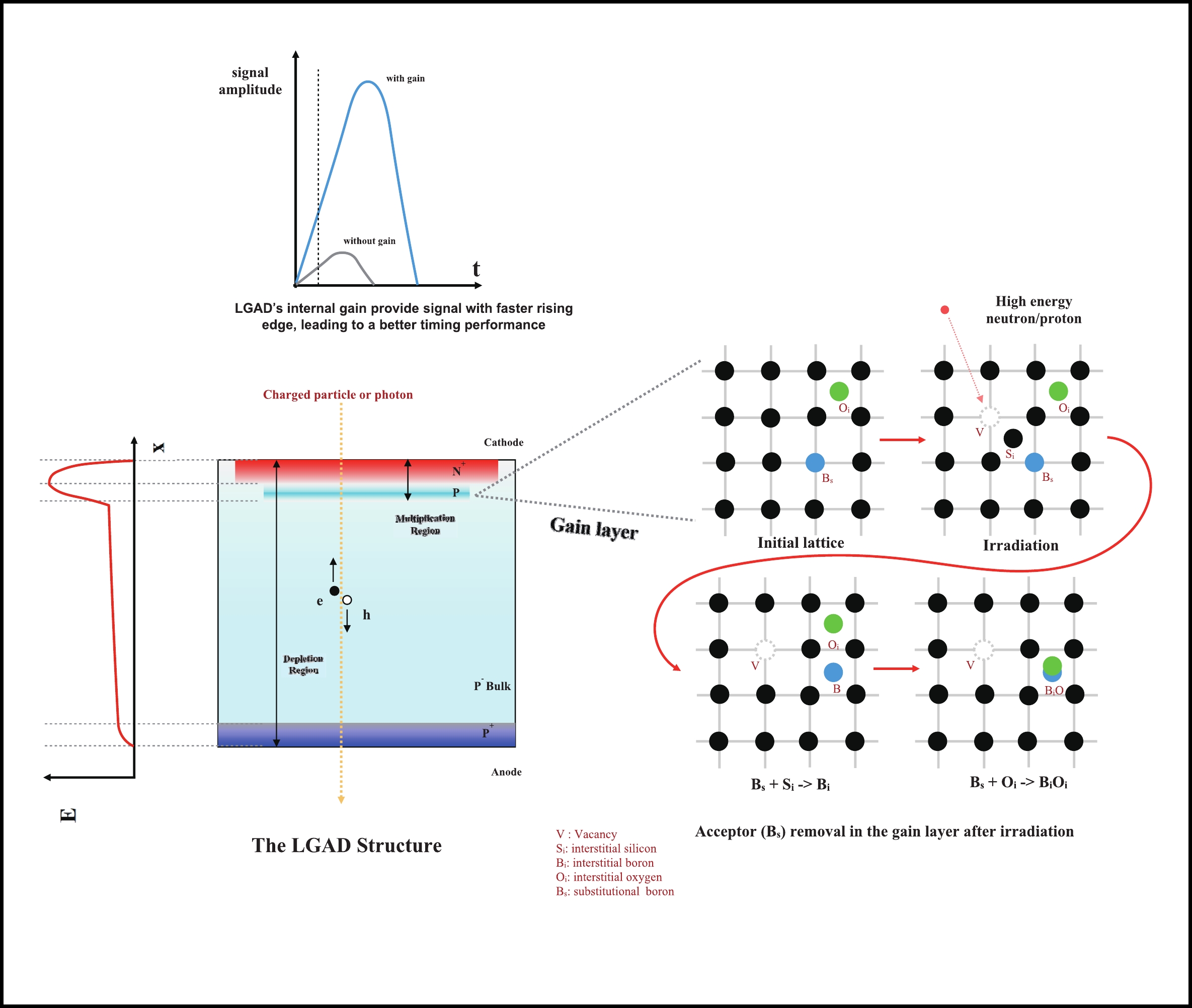
The basic principle and structure of the LGAD technology (left) and the acceptor removal effect (right) for the boron-doped gain layer. The BiOi complexes are generated after neutron/proton irradiation, leading to the reduction of the effective doping concentration and detector’s gain.
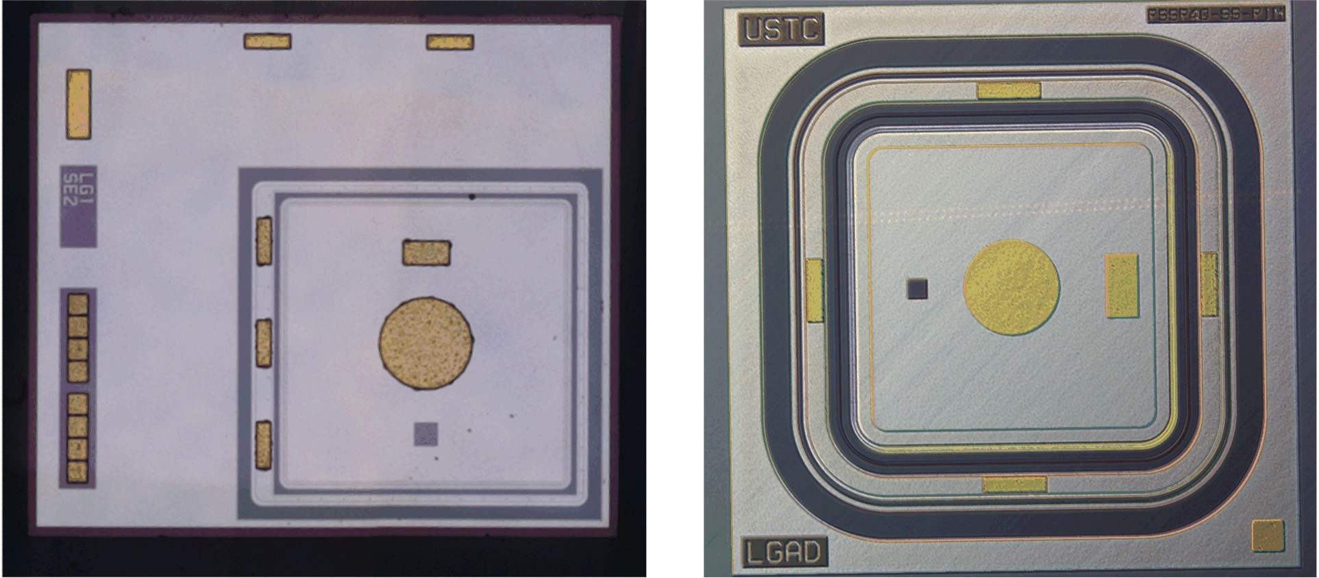
Figure 1. Photos of the HPK-1.2 (a) and USTC-1.1-W8 (b) single pad LGAD prototypes tested at USTC.
Figure 2. I-V results of the HPK-1.2, HPK-3.2 and USTC-1.1-W8 LGADs at difference fluences. The measurements are preformed at T = 20 ℃(room temperature) for all samples and T = −30 ℃ for USTC sensors with guard rings grounded.
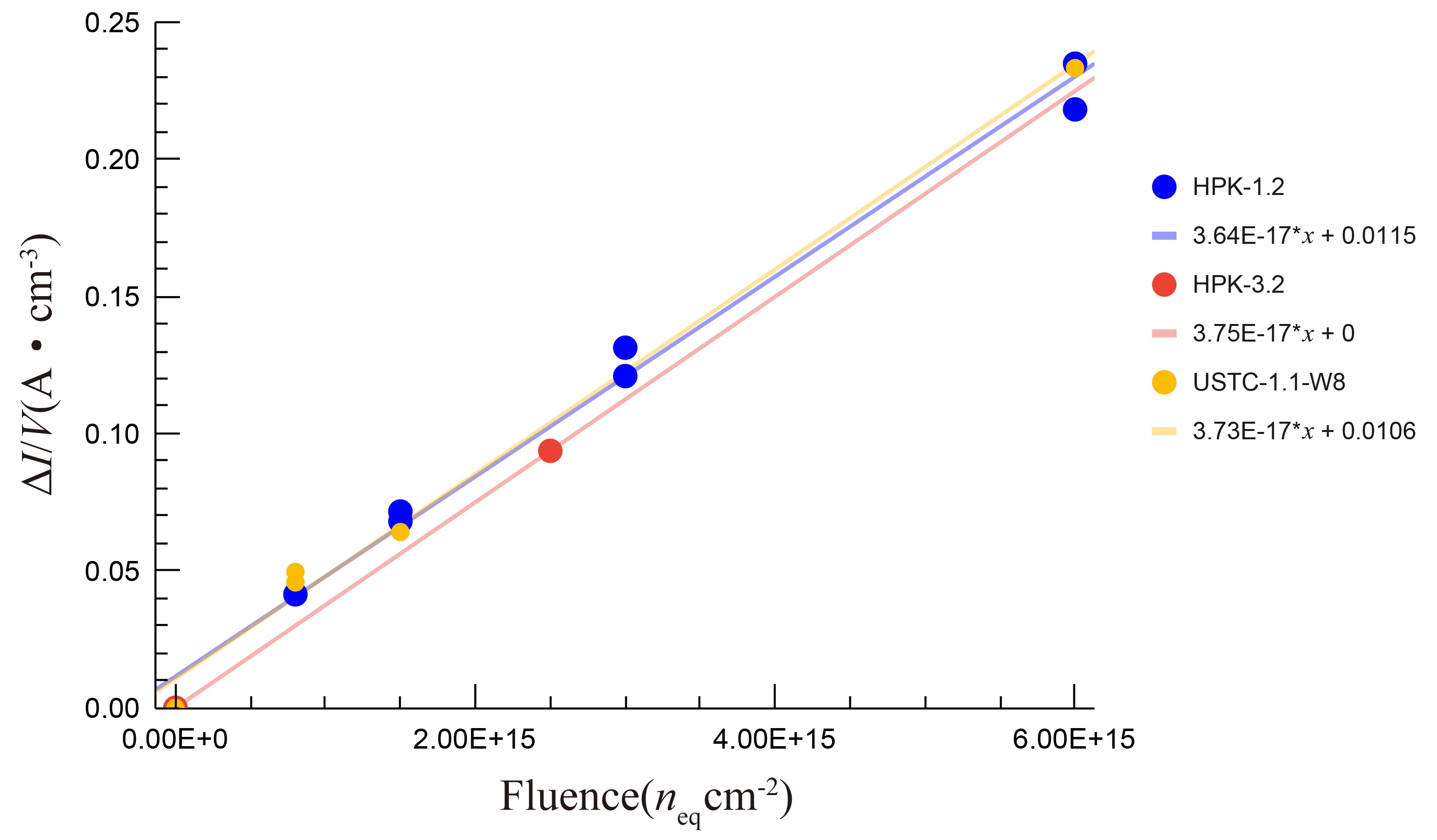
Figure 3. The ΔI/V at different fluences calculated from Room T. I-V for HPK-1.2, HPK-3.2 and USTC-1.1-W8 sensors used to estimate the α-factor representing the damages generated in the bulk region.
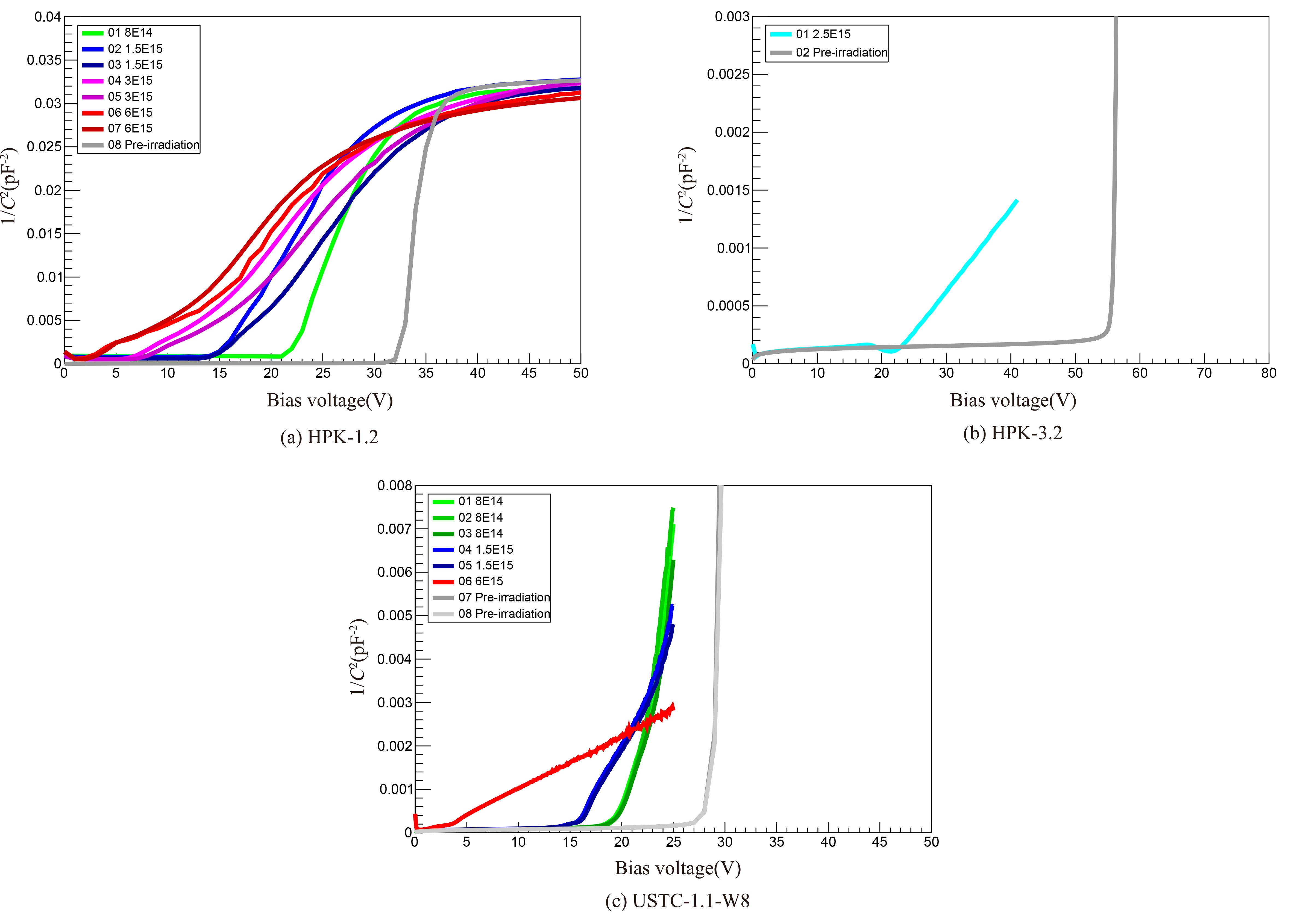
Figure 4. 1/C2 -V of the HPK-1.2, HPK-3.2 and USTC-1.1-W8 LGADs at difference fluences. The measurements are preformed at T = 20 ℃, with guard rings grounded.
Figure 7. Fraction of active acceptor dose changes with fluences measured from the room-temperature C-V. is shown as a function of fluences. The active acceptor density degrades significantly after 1E + 15.
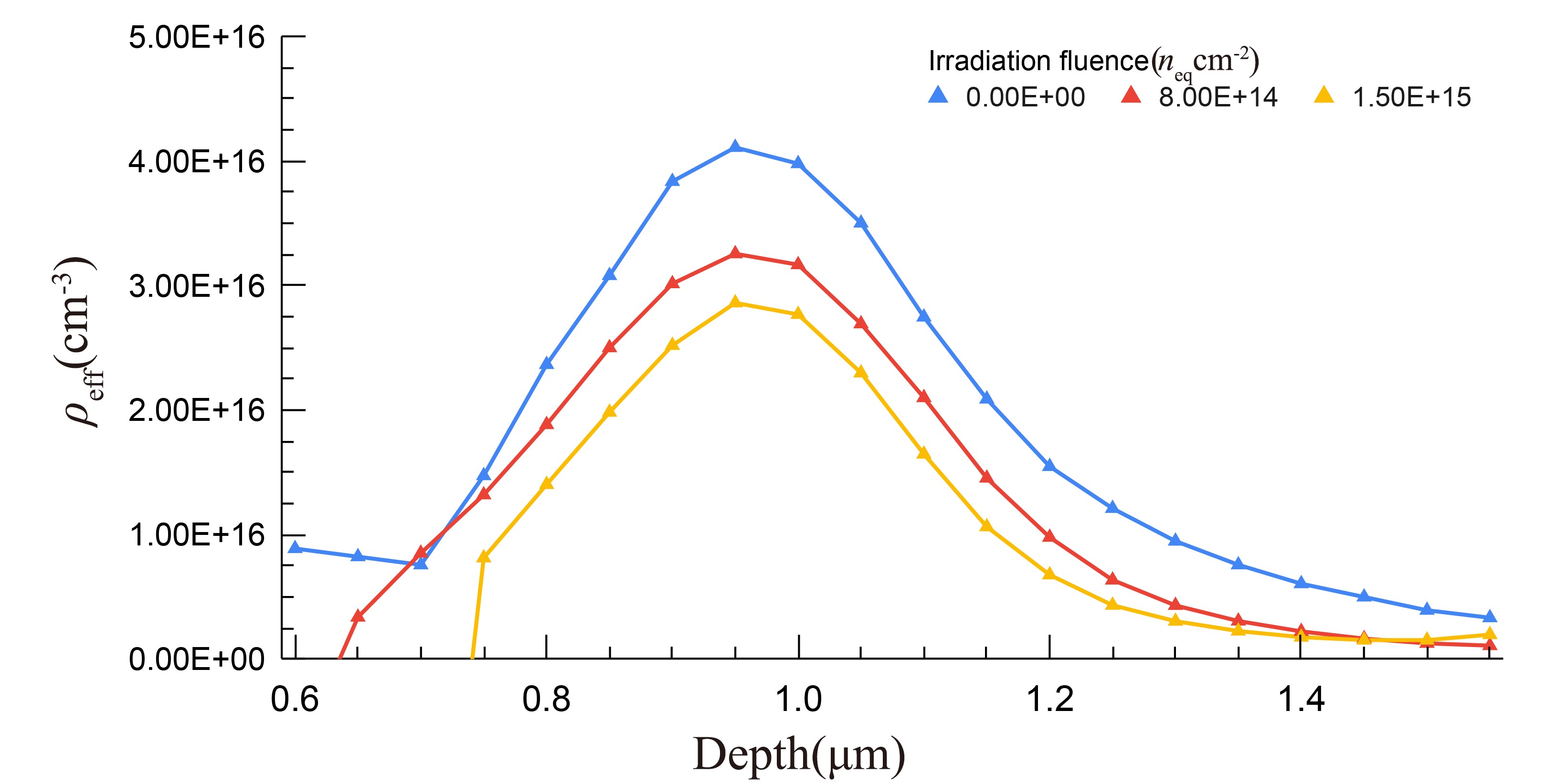
Figure 5. The doping profile before and after 8E+14, 1.5E+15 irradiation fluences of USTC-1.1-W8 LGAD samples. The doping density of each point is calculated by the average of the doping densities from the samples with the same fluence and average the results in each interval to suppress the fluctuation.
Figure 6. VGL as a function of fluences of all prototypes tested.
Figure 8. The c-factor as a function of initial doping density (ρ0) measured from USTC-1.1-W8 irradiated samples.
| [1] |
Pellegrini G, Fernández-Martínez P, Baselga M, et al. Technology developments and first measurements of Low Gain Avalanche Detectors (LGAD) for high energy physics applications. Nuclear Instruments and Methods in Physics Research A, 2014, 765: 12–16. DOI: 10.1016/j.nima.2014.06.008
|
| [2] |
Hartmann F. Evolution of Silicon Sensor Technology in Particle Physics. Berlin: Springer, 2017. https://linkspringer.53yu.com/book/10.1007%2F978-3-319-64436-3
|
| [3] |
Rd50 collaboration. RD50 - Radiation hard semiconductor devices for very high luminosity colliders. http://rd50.web.cern.ch/rd50.
|
| [4] |
Lanni F, Pontecorvo L. Technical design report: A high-granularity timing detector for the ATLAS Phase-Ⅱ Upgrade, Geneva, Switzerland: CERN, 2020.
|
| [5] |
Rossi L, Fischer P, Rohe T, et al. Pixel Detectors: From Fundamentals to Applications. Berlin: Springer, 2006. https://xs.dailyheadlines.cc/books?hl=zh-CN&lr=&id=Jbp73yTz-LYC&oi=fnd&pg=PA1&dq=Rossi+L,+Fischer+P,+Rohe+T,+et+al.+Pixel+Detectors:+From+Fundamentals+to+Applications.+Berlin:+Springer,+2006.&ots=YHP700x7Gt&sig=OxQfRU9rZumpdGwcgDKyBxDQHYc
|
| [6] |
Gurimskaya Y, de Almeida P D, Garcia M F, et al. Radiation damage in p-type EPI silicon pad diodes irradiated with protons and neutrons. Nuclear Instruments and Methods in Physics Research A, 2020, 958: 162221. DOI: 10.1016/j.nima.2019.05.062
|
| [7] |
Jin Y, Ren H, Christie S, et al. Experimental study of acceptor removal in UFSD. Nuclear Instruments and Methods in Physics Research A, 2020, 983: 164611. DOI: 10.1016/j.nima.2020.164611
|
| [8] |
Yang X, Alderweireldt S, Atanov N, et al. Layout and performance of HPK prototype LGAD sensors for the High-Granularity Timing Detector. Nuclear Instruments and Methods in Physics Research A, 2020, 980: 164379. DOI: 10.1016/j.nima.2020.164379
|
| [9] |
Shi X, Ayoub M K, Cui H, et al. Radiation campaign of HPK prototype LGAD sensors for the High-Granularity Timing Detector (HGTD). Nuclear Instruments and Methods in Physics Research A, 2020, 979: 164382. DOI: 10.1016/j.nima.2020.164382
|
| [10] |
Moll M. Radiation damage in silicon particle detectors. Hamburg, Germany: Hamburg University, 1999: DESY Thesis-1999-040. https://www.osti.gov/etdeweb/biblio/20033260
|
| [11] |
Snoj L, Ambrožič K, Čufar A, et al. Radiation hardness studies and detector characterisation at the JSI TRIGA reactor. EPJ Web of Conferences, 2020, 225: 04031. DOI: 10.1051/epjconf/202022504031
|
| [12] |
Moll M. Radiation damage and annealing in view of QA aspects. In: 1st Workshop on Quality Assurance Issues in Silicon Detectors. Geneva, Switzerland: CERN, 2001. http://ssd-rd.web.cern.ch/qa/talks/Michael_Moll-QA-2001.pdf
|
| [13] |
Wunstorf R. Systematic Studies on the Radiation Resistance of Silicon Detectors for the Application in High-Energy Physics Experiments. Hamburg, Germany: Deutsches Elektronen-Synchrotron (DESY), 1992. https://inis.iaea.org/search/search.aspx?orig_q=RN:24030522
|
| [14] |
Moll M, Fretwurst E, Lindström G, et al. Leakage current of hadron irradiated silicon detectors-material dependence. Nuclear Instruments and Methods in Physics Research A, 1999, 426: 87–93. DOI: 10.1016/S0168-9002(98)01475-2
|
| [15] |
Ferrero M, Arcidiacono R, Barozzi M, et al. Radiation resistant LGAD design. Nuclear Instruments and Methods in Physics Research A, 2019, 919: 16–26. DOI: 10.1016/j.nima.2018.11.121
|

ISSN 0253-2778
CN 34-1054/N
Copyright © Editorial Office of JUSTC, All Rights Reserved. 皖ICP备05002528号
Supported by: Beijing Renhe Information Technology Co., Ltd. 


 DownLoad: