Xianglu Wang is currently a master student at the School of Management, University of Science and Technology of China (USTC). He received his B.S. degree from USTC in 2019. His research mainly focuses on high-dimensional variable selection and inference
It is well known that regression methods designed for clean data will lead to erroneous results if directly applied to corrupted data. Despite the recent methodological and algorithmic advances in Gaussian graphical model estimation, how to achieve efficient and scalable estimation under contaminated covariates is unclear. Here a new methodology called convex conditioned innovative scalable efficient estimation (COCOISEE) for Gaussian graphical models under both additive and multiplicative measurement errors is developed. It combines the strengths of the innovative scalable efficient estimation in the Gaussian graphical model and the nearest positive semidefinite matrix projection, thus enjoying stepwise convexity and scalability. Comprehensive theoretical guarantees are provided and the effectiveness of the proposed methodology is demonstrated through numerical studies.
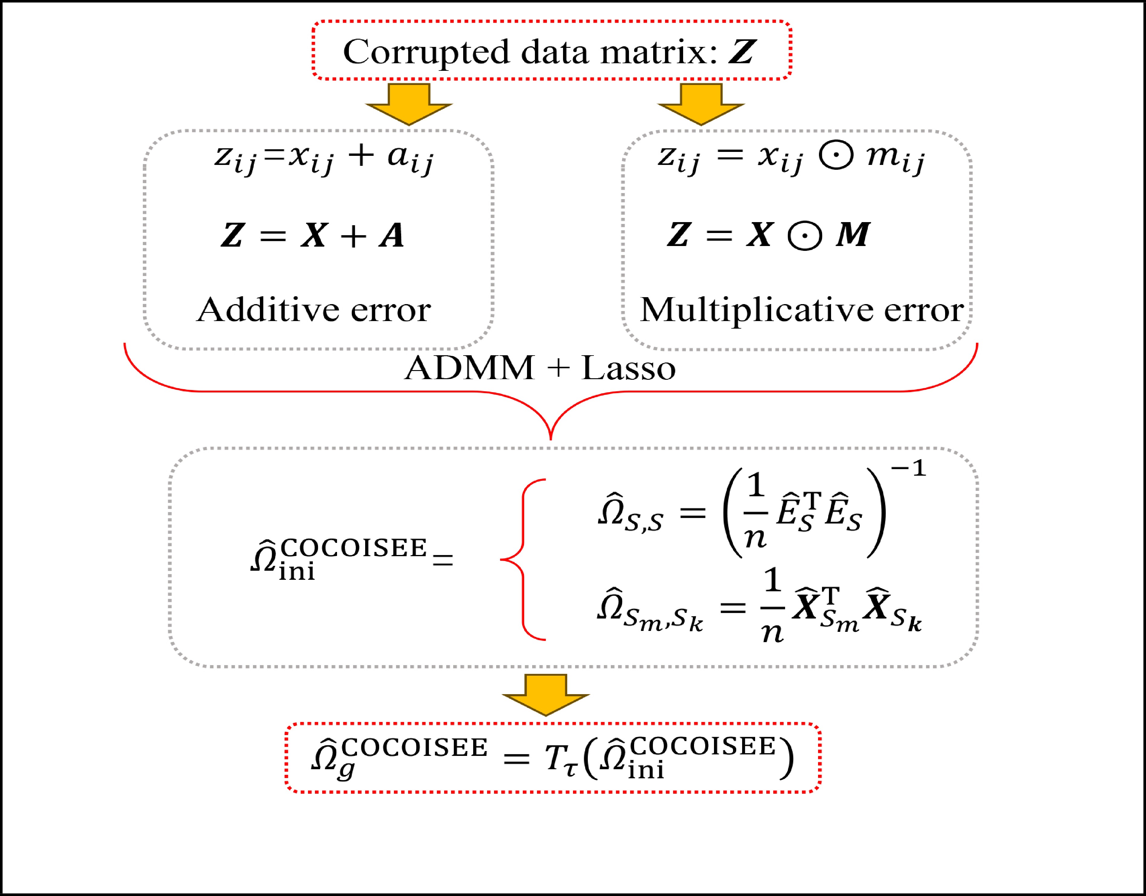
Graphical Abstract
The process of recovering the precision matrix in the presence of additive and multiplicative measurement errors.
Abstract
It is well known that regression methods designed for clean data will lead to erroneous results if directly applied to corrupted data. Despite the recent methodological and algorithmic advances in Gaussian graphical model estimation, how to achieve efficient and scalable estimation under contaminated covariates is unclear. Here a new methodology called convex conditioned innovative scalable efficient estimation (COCOISEE) for Gaussian graphical models under both additive and multiplicative measurement errors is developed. It combines the strengths of the innovative scalable efficient estimation in the Gaussian graphical model and the nearest positive semidefinite matrix projection, thus enjoying stepwise convexity and scalability. Comprehensive theoretical guarantees are provided and the effectiveness of the proposed methodology is demonstrated through numerical studies.
Public Summary
We propose a new methodology COCOISEE to achieve scalable and interpretable estimation for Gaussian graphical model under both additive and multiplicative measurement errors.
The method is stepwise convex, computationally stable, efficient and scalable.
Both theoretical and simulation results verify the feasibility of our method.
The estimation precision (inverse covariance) matrix has become a basic problem in modern multivariate statistical analysis and has a very wide range of practical applications. For example, in genome-wide association studies, genomic data are used to estimate the precision matrix and obtain the genetic correlation between traits from the nonzero terms. It is not only crucial for understanding gene regulatory pathways and gene functions but also contributes to a deeper understanding of the genetic basis of quantitative variation in complex traits[1]. Similarly, in social network analysis[2, 3], a precision matrix can be used to explore the correlation between users and is also widely used in economics and finance[4–6], health science[7], high-dimensional discriminant analysis[8], and complex data visualization[9].
The estimation of the precision matrix has attracted many scholars to study in recent years. In terms of the form of research methods, the currently proposed methods can be roughly divided into two classes: penalized likelihood methods and column-by-column estimation methods. The former class includes, for example, Ref. [10], which has laid down a general framework for the penalized likelihood method, and Refs. [11–15], which used different penalty algorithms to select zero elements in the precision matrix, and these methods all impose a penalty term on the negative log-likelihood function to estimate the precision matrix. The theoretical properties of these methods have been thoroughly studied by Refs. [16, 17]. The latter class includes, for instance, Refs. [8, 14, 18–21]. Such methods convert the problem of precision matrix estimation into a nodewise or pairwise regression, or optimization problem and then apply the technique of high-dimensional regularization using the Lasso or Dantzig selector type methods. However, most of these existing methods are designed for clean data, while corrupted data are often encountered in various fields. Naively applying the aforementioned methods to analyze the corrupted data can lead to inconsistent and unstable estimates, thus leading to misleading conclusions. Therefore, it is urgent to develop an efficient method for large precision matrix estimation under measurement errors.
Various statistical methods have been proposed to mitigate the effects of measurement errors. Specifically, there are a series of works to address measurement errors in univariate response linear regression models, which can be traced back to Ref. [22] and its extensions include Refs. [23, 24]. In recent years, great progress has also been made in high-dimensional error-in-variables regression. For instance, Ref. [25] developed a l1-regularized likelihood approach to handle missing data by solving a negative log-likelihood optimization problem via the EM algorithm. Similarly, Ref. [26] developed a Lasso-type estimator by replacing the corrupted Gram matrix with unbiased estimates for corrupted data. Furthermore, Ref. [27] proposed a Dantzig selector-type estimator based on the compensated matrix uncertainty method. However, after adjusting for corrupted data, negative likelihood functions are usually not convex and may depend on some crucial hidden parameters. To address this difficulty, Ref. [28] proposed the convex conditioned Lasso (CoCoLasso) method by replacing the unbiased covariance matrix estimate with the nearest positive semidefinite matrix, thus enjoying stepwise convexity in high-dimensional measurement error regression.
In this work, motivated by the study of the above scholars, we develop a new approach called convex conditioned innovative scalable efficient estimation (COCOISEE) to address Gaussian graphical models under measurement errors by combining the strengths of the recently developed innovative scalable efficient estimation[21] and the nearest positive semidefinite matrix projection[28], thus enjoying stepwise convexity and scalability.
The rest of the paper is organized as follows. Section 2 presents the model setting and the new methodology. Theoretical properties including consistency in estimation are established in Section 3. We provide simulation examples in Section 4. Section 5 discusses possible extensions of our method and possible future work. All technical details are relegated to Appendix.
Notation. We briefly summarize some symbols to be used throughout the paper. We use x, X, and X to denote vectors, elements, and matrices, respectively. For any matrix X=(Xij), let ‖ denote the matrix l_{\infty} norm, whereas \left \|{\boldsymbol{X}} \right \|_{\rm max}={\rm max}_{i, j}|X_{ij}| denotes the elementwise maximum norm. Similarly, for any vector {\boldsymbol{x}}=(X_1, ..., X_p)^{\rm T}, let ||{\boldsymbol{x}}||_q=\left( {\displaystyle \sum\limits_i|X_i|^q} \right)^{1/q} be the l_q norm of vector {\boldsymbol{x}}, and l_{\infty} vector norm is ||{\boldsymbol{x}}||_{\infty}={\rm max}_{i}|X_{i}|. For any subsets A, B \subset \{1, ..., p\} , denote by {\boldsymbol{x}}_A a subvector of {\boldsymbol{x}} formed by its components with indices in A , denote by {\boldsymbol{x}}_{-A} a subvector of {\boldsymbol{x}} formed by its components without indices in A , and \boldsymbol \varOmega_{A, B}=(w_{ij})_{i\in A, j\in B} a submatrix of {\boldsymbol \varOmega} with rows in A and columns in B. Let (S_{l})_{1\leqslant l \leqslant L} be a partition of the index set \{1, ..., p\} . \lambda_{\rm min}(\cdot) and \lambda_{\rm max}(\cdot) denote the smallest and largest eigenvalues of a given symmetric matrix, respectively. We use \varDelta to denote a fixed sequence going to zero.
2.
Gaussian graphical model under measurement errors
2.1
Model setting
Consider an undirected Gaussian graphical model G=(V, E) for a p -dimensional Gaussian random vector
where G is an undirected graph related to vector {\boldsymbol{x}}, V=\{X_1, ..., X_p\} is a node set, E=(e_{ij}) is an edge matrix with each entry e_{ij} representing the edge between X_i and X_j , \mu=(\mu_i)_{1\leqslant i \leqslant p} is a mean vector and \varSigma=(\sigma_{ij}) is a covariance matrix. Assume that \{{\boldsymbol{x}}_{i}\}_{1\leqslant i \leqslant n} is an independently identically distributed (\rm i.i.d.) sample from the Gaussian distribution. Without loss of generality, suppose that the mean vector \mu=0 throughout the paper. Denote by {\boldsymbol \varOmega} =(\omega_{ij}) the precision matrix, that is, the inverse \varSigma^{-1} of the covariance matrix \varSigma. It is well known that in Gaussian graphical model theory, an edge (i, j) exists (or e_{ij}\neq 0 ) between X_i and X_j if and only if the corresponding entry \omega_{ij} of the precision matrix is non-zero. The above characterization of the precision matrix shows that the problem of estimating Gaussian graphical model G can be equivalent to estimating the support:
To motivate our new method, we consider a linear transformation of the precision matrix similar to Ref. [21]. Specifically, based on the transformation of {\boldsymbol{x}}, we have the following structure:
Therefore, from the distribution of \tilde{{\boldsymbol{x}}}, we can see that if estimator \tilde{{\boldsymbol{x}}} is obtained, the precision matrix {\boldsymbol \varOmega} can be achieved by estimating the covariance matrix of \tilde{{\boldsymbol{x}}}.
By the definition of \tilde{{\boldsymbol{x}}}, we can write the subvector \tilde{{\boldsymbol{x}}}_{S} in following form:
where \varTheta_{S}=- {\boldsymbol \varOmega} _{-S, S} {\boldsymbol \varOmega} _{S, S}^{-1} is a n\times (p-|S|) dimensional regression coefficients matrix, and {\boldsymbol \eta}_{S}={\boldsymbol{x}}_{S}+ {\boldsymbol \varOmega} _{S, S}^{-1} {\boldsymbol \varOmega} _{S, -S}{\boldsymbol{x}}_{-S} is the matrix of model errors which has a multivariate Gaussian distribution N(0, {\boldsymbol \varOmega} _{S, S}^{-1}) and independent of {\boldsymbol{x}}_{-S}. Thus, the estimates of the two terms on the right side of Eq. (2) are correlated and can be efficiently achieved by linear regression techniques, i.e., Lasso[29].
The representation of subvector {\boldsymbol{x}}_{S} shows that the unknown subvector \tilde{{\boldsymbol{x}}}_{S} can be estimated by the regression technique. To see this, let \hat{{\boldsymbol \eta}}_{S} be the residual vector obtained by fitting model (4) using Lasso. Then the unknown matrix {\boldsymbol \varOmega} _{S, S} can be estimated as the inverse of the sample covariance matrix of the model residual vector \hat{{\boldsymbol \eta}}_{S} . Then we can estimate the subvector \tilde{{\boldsymbol{x}}}_{S} in Eq. (2) as \hat{{\boldsymbol{x}}}_{S}=\hat{ {\boldsymbol \varOmega} }_{S, S}\hat{{\boldsymbol \eta}}_{S}.
The ISEE[21] repeated the above procedure for each S_{l} with 1\leqslant l \leqslant p to obtain the estimated subvectors \hat{{\boldsymbol{x}}}_{S_{l}}’s, and then stacked all these subvectors together to form an estimate \hat{{\boldsymbol{x}}} of the oracle innovated vector \tilde{{\boldsymbol{x}}}. Thus, the problem of estimating the precision matrix based on the original vector {\boldsymbol{x}} reduces to that of estimating the covariance matrix based on the estimated transformed vector \tilde{{\boldsymbol{x}}}.
However, in many practical applications, the data we collect may contain unobvious measurement errors, resulting in inaccurate Gaussian graphical model estimation. In this paper, we consider two kinds of measurement errors associated with matrix {\boldsymbol{X}}, as shown below:
● Additive error. We assume that the observed elements of the data matrix \boldsymbol{Z} are affected by additive measurement errors z_{ij}=x_{ij}+a_{ij} , and write it as a matrix form \boldsymbol{Z}= \boldsymbol{X} + \boldsymbol{A}, where {\boldsymbol{A}}= (a_{ij})_{p\times p} is the measurement error matrix. We assume that the rows of \boldsymbol{A} are \rm i.i.d. with mean \bf{0} and finite covariance matrix \varSigma^{A}.
● Multiplicative error. We assume that the observed elements of the data matrix {\boldsymbol{Z}} are affected by multiplicative measurement errors z_{ij}= x_{ij} \odot m_{ij} , and write it as a matrix form \boldsymbol{Z}= \boldsymbol{X} \odot \boldsymbol{M}, where \odot denotes the Hadamard product and {\boldsymbol{M}} = (m_{ij})_{p\times p} is the measurement error matrix. We also assume that the rows of {\boldsymbol{M}} are \rm i.i.d. with mean \boldsymbol{\mu^{M}} and finite covariance matrix \varSigma^{M}. Particularly, missing data can be regarded as a special case of the multiplicative measurement error, where m_{ij}=I(x_{ij}) , and I(\cdot) represents the indicator function.
2.2
Scalable estimation by COCOISEE
The data matrix is denote by {\boldsymbol{X}}=({\boldsymbol{x}}_{1}, ..., {\boldsymbol{x}}_{n})^{\rm T}\in {\rm R}^{n\times p}. Then, the transformed data matrix is defined as \tilde{{\boldsymbol{X}}}={\boldsymbol{X}} {\boldsymbol \varOmega} . Thus, Eq. (4) can be rewritten as
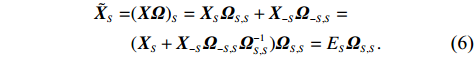
where E_{S} is an error matrix with rows being \rm i.i.d. copies from {\boldsymbol \eta}_{S}^{\rm T}. Then, \tilde{{\boldsymbol{X}}}_{S} can be written as
The representation in Eq. (6) provides the basis for the estimation of matrix \tilde{{\boldsymbol{X}}}.
To fit the Gaussian linear regression model (5), we suggest univariate regression methods. Specifically, for each node i in the index set S , we consider the univariate linear regression model for {\boldsymbol{X}}_{i} :
In general, we can use some high-dimensional regression methods to fit Eq. (7), such as SCAD[30], Lasso[29], elastic net[31], adaptive Lasso[32], and Dantzig selector[33]. However, we observe the data matrix {\boldsymbol{Z}} instead of the matrix {\boldsymbol{X}} in linear models with error-in-variables. Thus, directly applying Lasso to this equation by minimizing
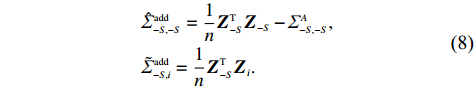
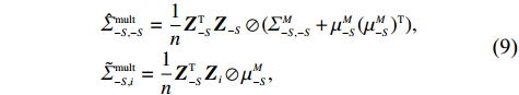
is often erroneous, where \varSigma_{-S, -S}=\dfrac{1}{n}{\boldsymbol{Z}}_{-S}^{\rm T}{\boldsymbol{Z}}_{-S} and \varSigma_{-S, i}= \dfrac{1}{n}{\boldsymbol{Z}}_{-S}^{\rm T}{\boldsymbol{Z}}_{i}. Based on the corrupted data matrix {\boldsymbol{Z}} , Ref. [28] suggested constructing unbiased surrogates \hat{\varSigma}_{-S, -S} and \tilde{\varSigma}_{-S, i} for \varSigma_{-S, -S} and \varSigma_{-S, i} that cannot be observed to mitigate the effects of measurement errors. For the additive error setting, the unbiased surrogates are defined as
where \oslash represents the element division operator of vectors and matrices. Since \varSigma^{A} or (\varSigma^{M}, \mu^{M}) can be obtained in practice through repeated measurements or field experience, we assume that they are known for the model.
However, the estimator \hat{\varSigma} is usually not positive semidefinite in high-dimensional models, resulting in the related optimization problems that may no longer be convex. To overcome this problem, we draw on the idea of Ref. [28] to obtain the sparse regression coefficients \theta_{i} by minimizing
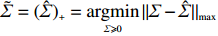
where \tilde{\varSigma}_{-S, -S} is the principal submatrix of \tilde{\varSigma}, and \tilde{\varSigma}=(\hat{\varSigma})_{+}=\mathop{\rm argmin}\limits_{\varSigma \geqslant 0}||\varSigma-\hat{\varSigma}||_{\rm max} is the nearest positive semidefinite matrix. From the definition of \tilde{\varSigma}, we can solve it efficiently by an alternating direction method of multipliers (ADMM) and have
Eq. (11) is obtained by the triangle inequality and the definition of \tilde{\varSigma} ensures \tilde{\varSigma} approximates \varSigma as well as the initial surrogate \hat{\varSigma}.
Based on the regression step, for each node i in the index set S we cannot directly replace {\boldsymbol{Z}} with {\boldsymbol{X}} in Eq. (5) to calculate \hat{E}_{S} . Instead, we can use \hat{E}_{S} as an intermediate variable to calculate \hat {\boldsymbol \varOmega} _{S, S}.Then the estimator \hat {\boldsymbol \varOmega} _{S, S} can be written as
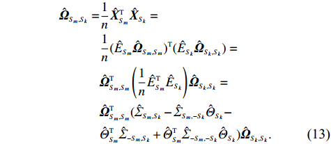
where \hat{\varTheta}_{S}=(\hat{\theta}_{i})_{i\in S}. These observations suggest a simple plug-in estimator \hat{E}_{S}\hat{ {\boldsymbol \varOmega} }_{S, S} for the unobservable submatrix \hat{{\boldsymbol{X}}}_{S} in Eq. (6). Since the error matrix \hat{E}_{S} is unknown, we cannot directly calculate \hat{{\boldsymbol{X}}}_{S}. Similarly, for each 1\leqslant k \neq m \leqslant L, we can use \hat{{\boldsymbol{X}}}_{S_{k}} and \hat{{\boldsymbol{X}}}_{S_{m}} as intermediate variables to calculate \hat{ {\boldsymbol \varOmega} }_{S_{m}, S_{k}}. Then the estimator \hat{ {\boldsymbol \varOmega} }_{S_{m}, S_{k}} can be written as
where T_{\tau}({\boldsymbol{X}})=(x_{ij}I_{|x_{ij}|\geqslant \tau}) denotes the matrix {\boldsymbol{X}} thresholded at \tau . Thus, the set of links of graphical structure is {\rm supp}(\hat{ {\boldsymbol \varOmega} }_{g}^{\rm COCOISEE}). The choice of the threshold \tau in Eq. (15) is important for practical implementation. We use the cross-validation method for large precision matrix estimation. Specifically, we randomly split the sample of n rows of the sample matrix {\boldsymbol{Z}} into two subsamples of sizes n_1 and n_2 , and repeat this R times. Denote by \hat{ {\boldsymbol \varOmega} }_{\rm ini}^{\rm COCOISEE}(n_{1}, i) and \hat{ {\boldsymbol \varOmega} }_{\rm ini}^{\rm COCOISEE}(n_{2}, i) the precision matrices as defined in Eq. (14) based on these two subsamples, respectively, for the i th split. Thus, the threshold \tau can be chosen to minimize
In this section, we will present several technical conditions and then analyze the theoretical properties of COCOISEE.
3.1
Technical conditions
Condition 1. (Closeness condition) Assume that the distributions of \hat{\varSigma}_{-S, -S} and \tilde{\varSigma}_{-S, j} are identified by a set of parameters \theta . Then there exist universal constants C and c , and positive functions \zeta and \epsilon_0 depending on \theta and \sigma^2 such that for any \varepsilon\leqslant \varepsilon_0, \hat{\varSigma}_{-S, -S} and \tilde{\varSigma}_{-S, j} satisfy the following probability statements:
\begin{split} &{\rm Pr}(|(\hat{\varSigma}_{-S, -S})_{ij}-(\varSigma_{-S, -S})_{ij}|\geqslant \varepsilon)\leqslant C {\rm exp}(-cn\varepsilon^{2}\zeta^{-1}) ,\quad \\&\forall i, j\in(\{1, ..., p\}-S). \end{split}
Condition 2. (Restricted eigenvalue condition) The restricted eigenvalue of the Gram matrix \varSigma=\dfrac{1}{n}{\boldsymbol{X}}^{\rm T}{\boldsymbol{X}} satisfies:
where \kappa=\{1, ..., K\} is the true support set of the regression coefficient vector \theta^{*} .
Condition 4. The entries of measurement error matrices A and M are all independent and identically distributed sub-Gaussian random variables.
Condition 5. The random vectors {\boldsymbol \eta}_{i} obey a zero-mean sub-Gaussian distribution with a finite variance parameter, i.e., \sigma_{i}^{2}\leqslant C.
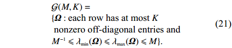
Condition 6. The Gaussian graph model we focus on satisfies the following conditions.
Condition 1 ensures that the surrogates \hat{\varSigma}_{-S, -S} (and hence \tilde{\varSigma}_{-S, -S}) and \hat{\varSigma}_{-S, j} are close to \varSigma_{-S, -S} and \varSigma_{-S, j} respectively in terms of the elementwise maximum norm. Condition 2 is the restricted eigenvalue condition proposed in Ref. [34], and is widely used in Lasso related articles. It imposes a lower bound on eigenvalues of the Gram matrix \varSigma to constrain the correlations between relatively small numbers of predictors in the design matrix {\boldsymbol{X}} . Condition 3 is the irrepresentable condition proposed in Refs. [35, 36], and was obtained to prove a model selection consistency result for Gaussian graphical model selection using the Lasso. Conditions 1–3 are necessary conditions for proving Lemma A.1 introduced in Appendix.
Condition 4 imposes a mild assumption on measurement error matrices since sub-Gaussians are a natural kind of random variable for which the properties of Gaussians can be extended[37]. Condition 5 is standard and has been widely used in high-dimensional linear regression models. Condition 6 guarantees that the number of links for each node is bounded by K from above and that the precision matrix has a bounded spectrum[21].
3.2
Main results
Theorem 1. Assume that Conditions 1–6 hold and \lambda K\to o(1) . Then with probability 1- \varDelta tending to one the initial COCOISEE estimator \hat{ {\boldsymbol \varOmega} }_{\rm ini}^{\rm COCOISEE} in Eq. (14) satisfies that
Theorem 1 establishes the entrywise infinity norm estimation bound for the initial COCOISEE estimator. From the proof of Theorem 1 in Appendix, we see that the rate of convergence for the initial COCOISEE estimator is the maximum of two components \lambda^{2}K and \lambda for both block-diagonal and off-block-diagonal entries of \hat{ {\boldsymbol \varOmega} }_{\rm ini}^{\rm COCOISEE}. Since we assume that \lambda K\to o(1) , the rate of convergence O(\lambda) dominates that of O(\lambda^2 K) , meaning that the rate of convergence for the initial COCOISEE estimator is change into O(\lambda) .
Theorem 2. Assume that the conditions of Theorem 1 hold and \omega_{0}={\rm min}\{|\omega_{jk}|:(j, k)\in {\rm supp} ( {\boldsymbol \varOmega} )\}\geqslant \omega_{0}^{*}=C\lambda with C>0 and some sufficiently large constants. Then, with probability 1-\varDelta tending to one, and for any \tau\in[c\omega_{0}^{*}, \omega_{0}-c\omega_{0}^{*}] with c\in (0, {1}/{2}), we have
Theorem 2 shows that the sparse precision matrix estimator \hat{ {\boldsymbol \varOmega} }_{g}^{\rm COCOISEE} enjoy good asymptotic properties.
4.
Simulation studies
In this section, we simulated the finite-sample performance of the proposed COCOISEE method. To illustrate the impact of ignoring measurement errors, we compared two methods designed for clean data sets: Glasso[12] and ISEE[21]. The three methods were implemented as follows. Glasso was implemented by the R package glasso and had a tuning parameter that was chosen using five-fold cross-validation. ISEE[21] selected the tuning parameters in scaled Lasso[38] following the suggestion of Ref. [39] and adapted the cross-validation method proposed in Refs. [40, 41] for the threshold parameters. For the implementation of our COCOISEE approach, we used 5-fold corrected cross-validation, similar to Ref. [29]. Specifically, we used 90 \% of the sample to calculate \hat{ {\boldsymbol \varOmega} }_{\rm ini}^{\rm COCOISEE}(n_{1}, i) and the remained 10 \% to calculate \hat{ {\boldsymbol \varOmega} }_{\rm ini}^{\rm COCOISEE}(n_{2}, i). Then, we choose \tau from 20 values with the same interval by minimizing criterion (16) with the number of random splits set to R=5 .
We generated 50 data sets. For each data set, we generate the precision matrix {\boldsymbol \varOmega} in two steps. First, we produce a band matrix {\boldsymbol \varOmega} _{0} with diagonal entries being one, {\boldsymbol \varOmega} _{0}(i, i+1)= {\boldsymbol \varOmega} _{0}(i+1, i)=0.5 for i=1, ..., p , and all other entries being zero. Second, we randomly permute the rows and columns of {\boldsymbol \varOmega} _{0} to obtain the precision matrix {\boldsymbol \varOmega} . Thus, in general, the final precision matrix {\boldsymbol \varOmega} no longer has the band structure. We next sample the rows of the n\times p data matrix {\boldsymbol{X}} as i.i.d. vectors copied from the multivariate Gaussian distribution N(0, {\boldsymbol \varOmega} ^{-1}). Then, based on different types of measurement errors, the corrupted covariate matrices {\boldsymbol{Z}} can be provided respectively as follows.
● Additive errors case. The observed covariates \boldsymbol{Z}={\boldsymbol{X}}+{\boldsymbol A}, where the rows of {\boldsymbol{A}} are i.i.d. vectors copied from N(0, \tau^{2}) with \tau=0.2 .
● Multiplicative errors case. The observed covariates are \boldsymbol{Z}={\boldsymbol X}\odot {\boldsymbol M}, where the elements of \boldsymbol{M} follow a log-normal distribution, meaning that {\rm log} (m_{ij})’s are i.i.d. variables from N(0, \tau^{2}) with \tau=0.2 .
● Missing data case. The observed covariates are defined as z_{ij}=x_{ij}m_{ij} , where m_{ij}=I(x_{ij}{\text{ is not missing}}) , so that the covariates are missing at random with probability 0.1.
Due to high computational cost, we consider settings with n=100 , whose dimensionality p varies in \{50, 100, 150, 200\} .
To compare the aforementioned methods, we consider the same performance measures as suggested in Ref. [21]. The first two measures are the true positive rate (TPR) and the false positive rate (FPR), defined as
Tables 1–3 summarize the simulation results of these three performance measures for additive, multiplicative error and missing data cases. In view of TPR, FPR, and NEE in these tables, it is clear that the NEE of COCOISEE is the best, and both TPR and FPR are also doing very well.
In this paper, we have introduced a new methodology COCOISEE to achieve scalable and interpretable estimation for a Gaussian graphical model under both additive and multiplicative measurement errors. It takes full advantage of recently developed innovative scalable efficient estimation and the nearest positive semidefinite matrix projection, thus enjoying stepwise convexity and scalability in Gaussian graphical model estimation. The suggested method is ideal for parallel and distributed computing and cloud computing and has been shown to enjoy appealing theoretical properties. Both the established theoretical properties and numerical performances demonstrate that the proposed method enjoys good estimation, recovery accuracy, and high scalability under both additive and multiplicative measurement errors. Similar theoretical conclusions can also be extended to random sub-Gaussian settings. It would be very interesting to study several extensions of COCOISEE to more general model settings such as the time series model, the generalized linear model and the large nonparanormal graphical model, which are beyond the scope of the current paper and demand future studies.
There are three main contributions in this paper. First, the proposed COCOISEE method has scalability and high efficiency, because the main calculation cost comes from the estimation of the regression coefficient in the case of measurement error, and the other steps adopt matrix operation, which has relatively high calculation efficiency. Second, we use a recently developed semipositive definite matrix projection technique to mitigate the effects of measurement errors when recovering high-dimensional coefficient matrices from column-by-column regression. Therefore, COCOISEE enjoys progressive convexity and computational stability. Finally, we provide comprehensive theoretical properties to the proposed method by establishing the consistency of the estimator. Numerical results show the effectiveness of the proposed method.
Conflict of interest
The author declares that he has no conflict of interest.
Conflict of Interest
The authors declare that they have no conflict of interest.
We propose a new methodology COCOISEE to achieve scalable and interpretable estimation for Gaussian graphical model under both additive and multiplicative measurement errors.
The method is stepwise convex, computationally stable, efficient and scalable.
Both theoretical and simulation results verify the feasibility of our method.
Baselmans B M, Jansen R, Ip H F, et al. Multivariate genome-wide analyses of the well-being spectrum. Nature Genetics,2019, 51 (3): 445–451. DOI: 10.1038/s41588-018-0320-8
[2]
Yang K, Lee L F. Identification and QML estimation of multivariate and simultaneous equations spatial autoregressive models. Journal of Econometrics,2017, 196 (1): 196–214. DOI: 10.1016/j.jeconom.2016.04.019
[3]
Zhu X, Huang D, Pan R, et al. Multivariate spatial autoregressive model for large scale social networks. Journal of Econometrics,2020, 215 (2): 591–606. DOI: 10.1016/j.jeconom.2018.11.018
[4]
Han F, Liu H. Optimal rates of convergence for latent generalized correlation matrix estimation in transelliptical distribution. arXiv: 1305.6916, 2013.
[5]
Rubinstein M. Markowitz’s “portfolio selection”: A fifty-year retrospective. The Journal of Finance,2002, 57 (3): 1041–1045. DOI: 10.1111/1540-6261.00453
[6]
Wegkamp M, Zhao Y. Adaptive estimation of the copula correlation matrix for semiparametric elliptical copulas. Bernoulli,2016, 22 (2): 1184–1226. DOI: 10.3150/14-BEJ690
[7]
Fan J, Han F, Liu H. Challenges of big data analysis. National Science Review,2014, 1 (2): 293–314. DOI: 10.1093/nsr/nwt032
[8]
Cai T, Liu W, Luo X. A constrained ℓ1 minimization approach to sparse precision matrix estimation. Journal of the American Statistical Association,2011, 106 (494): 594–607. DOI: 10.1198/jasa.2011.tm10155
[9]
Tokuda T, Goodrich B, van Mechelen I, et al. Visualizing distributions of covariance matrices. New York: Columbia University, 2011.
[10]
Fan J, Peng H. Nonconcave penalized likelihood with a diverging number of parameters. The Annals of Statistics,2004, 32 (3): 928–961. DOI: 10.1214/009053604000000256
[11]
Yuan M, Lin Y. Model selection and estimation in the Gaussian graphical model. Biometrika,2007, 94 (1): 19–35. DOI: 10.1093/biomet/asm018
[12]
Friedman J, Hastie T, Tibshirani R. Sparse inverse covariance estimation with the graphical Lasso. Biostatistics,2008, 9 (3): 432–441. DOI: 10.1093/biostatistics/kxm045
[13]
Banerjee O, El Ghaoui L, d’Aspremont A. Model selection through sparse maximum likelihood estimation for multivariate Gaussian or binary data. The Journal of Machine Learning Research,2008, 9: 485–516. DOI: 10.5555/1390681.1390696
[14]
Meinshausen N, Bühlmann P. High-dimensional graphs and variable selection with the Lasso. The Annals of Statistics,2006, 34 (3): 1436–1462. DOI: 10.1214/009053606000000281
[15]
Wille A, Zimmermann P, Vranova E, et al. Sparse graphical Gaussian modeling of the isoprenoid gene network in Arabidopsis thaliana. Genome Biology,2004, 5 (11): R92. DOI: 10.1186/gb-2004-5-11-r92
[16]
Rothman A J, Bickel P J, Levina E, et al. Sparse permutation invariant covariance estimation. Electronic Journal of Statistics,2008, 2: 494–515. DOI: 10.1214/08-EJS176
[17]
Lam C, Fan J. Sparsistency and rates of convergence in large covariance matrix estimation. The Annals of Statistics,2009, 37 (6B): 4254–4278. DOI: 10.1214/09-AOS720
[18]
Yuan M. High dimensional inverse covariance matrix estimation via linear programming. The Journal of Machine Learning Research,2010, 11: 2261–2286. DOI: 10.5555/1756006.1859930
[19]
Liu W, Luo X. High-dimensional sparse precision matrix estimation via sparse column inverse operator. arXiv: 1203.3896, 2012.
[20]
Sun T, Zhang C H. Sparse matrix inversion with scaled Lasso. The Journal of Machine Learning Research,2013, 14 (1): 3385–3418. DOI: 10.5555/2567709.2567771
[21]
Fan Y, Lv J. Innovated scalable efficient estimation in ultra-large Gaussian graphical models. The Annals of Statistics,2016, 44 (5): 2098–2126. DOI: 10.1214/15-AOS1416
[22]
Bickel P, Ritov Y. Efficient estimation in the errors in variables model. The Annals of Statistics,1987, 15 (2): 513–540. DOI: 10.1214/aos/1176350358
[23]
Ma Y, Li R. Variable selection in measurement error models. Bernoulli,2010, 16 (1): 274–300. DOI: 10.3150/09-bej205
[24]
Liang H, Li R. Variable selection for partially linear models with measurement errors. Journal of the American Statistical Association,2009, 104 (485): 234–248. DOI: 10.1198/jasa.2009.0127
[25]
Städler N, Bühlmann P. Missing values: Sparse inverse covariance estimation and an extension to sparse regression. Statistics and Computing,2012, 22 (1): 219–235. DOI: 10.1007/s11222-010-9219-7
[26]
Loh P L, Wainwright M J. High-dimensional regression with noisy and missing data: Provable guarantees with nonconvexity. Advances in Neural Information Processing Systems,2012, 40 (3): 1637–1664. DOI: 10.1214/12-AOS1018
[27]
Belloni A, Rosenbaum M, Tsybakov A B. Linear and conic programming estimators in high dimensional errors-in-variables models. Journal of the Royal Statistical Society: Series B (Statistical Methodology),2017, 79 (3): 939–956. DOI: 10.1111/rssb.12196
[28]
Datta A, Zou H. Cocolasso for high-dimensional error-in-variables regression. The Annals of Statistics,2017, 45 (6): 2400–2426. DOI: 10.1214/16-AOS1527
[29]
Tibshirani R. Regression shrinkage and selection via the Lasso. Journal of the Royal Statistical Society: Series B (Methodological),1996, 58 (1): 267–288. DOI: 10.1111/j.2517-6161.1996.tb02080.x
[30]
Fan J, Li R. Variable selection via nonconcave penalized likelihood and its oracle properties. Journal of the American Statistical Association,2001, 96 (456): 1348–1360. DOI: 10.1198/016214501753382273
[31]
Zou H, Hastie T. Regularization and variable selection via the elastic net. Journal of the Royal Statistical Society: Series B (Statistical Methodology),2005, 67 (2): 301–320. DOI: 10.1111/j.1467-9868.2005.00503.x
[32]
Zou H. The adaptive Lasso and its oracle properties. Journal of the American Statistical Association,2006, 101 (476): 1418–1429. DOI: 10.1198/016214506000000735
[33]
Candes E, Tao T. The Dantzig selector: Statistical estimation when p is much larger than n. The Annals of Statistics,2007, 35 (6): 2313–2351. DOI: 10.1214/009053606000001523
[34]
Bickel P J, Ritov Y, Tsybakov A B. Simultaneous analysis of Lasso and Dantzig selector. The Annals of Statistics,2009, 37 (4): 1705–1732. DOI: 10.1214/08-AOS620
[35]
Zhao P, Yu B. On model selection consistency of Lasso. The Journal of Machine Learning Research,2006, 7: 2541–2563. DOI: 10.5555/1248547.1248637
[36]
Wainwright M J. Sharp thresholds for high-dimensional and noisy sparsity recovery using l1-constrained quadratic programming (Lasso). IEEE Transactions on Information Theory,2009, 55 (5): 2183–2202. DOI: 10.1109/TIT.2009.2016018
[37]
Buldygin V V, Kozachenko Yu V. Metric Characterization of Random Variables and Random Processes. Providence, RI: American Mathematical Society, 2000.
[38]
Sun T, Zhang C H. Scaled sparse linear regression. Biometrika,2012, 99 (4): 879–898. DOI: 10.1093/biomet/ass043
[39]
Ren Z, Sun T, Zhang C H, et al. Asymptotic normality and optimalities in estimation of large Gaussian graphical models. The Annals of Statistics,2015, 43 (3): 991–1026. DOI: 10.1214/14-AOS1286
[40]
Bickel P J, Levina E. Regularized estimation of large covariance matrices. The Annals of Statistics,2008, 36 (1): 199–227. DOI: 10.1214/009053607000000758
[41]
Bickel P J, Levina E. Covariance regularization by thresholding. The Annals of Statistics,2008, 36 (6): 2577–2604. DOI: 10.1214/08-AOS600


 DownLoad: