Siyu Jiang is currently a graduate student under the tutelage of Prof. Hong Zhang at the University of Science and Technology of China. His research mainly focuses on statistical genetics
Hong Zhang is a Full Professor at the University of Science and Technology of China (USTC). He received his Bachelor’s degree in Mathematics and Ph.D. degree in Statistics from USTC in 1997 and 2003, respectively. His research mainly focuses on statistical genetics, causal inference, and machine learning
In the interdisciplinary realm of statistics, genetics, and epidemiology, longitudinal sibling pair data offers a unique perspective for investigating complex diseases and traits, allowing the exploration of the dynamic processes of gene expression over time by controlling numerous confounding factors. Missing-not-at-random (MNAR) data are commonly used in such types of studies, but no statistical methods specifically tailored have been developed to handle MNAR data in complex longitudinal data in the literature. Here, we propose a new statistical method by jointly modeling longitudinal data from sib-pairs and MNAR data. Extensive simulations demonstrate the excellent finite sample properties of the proposed method.
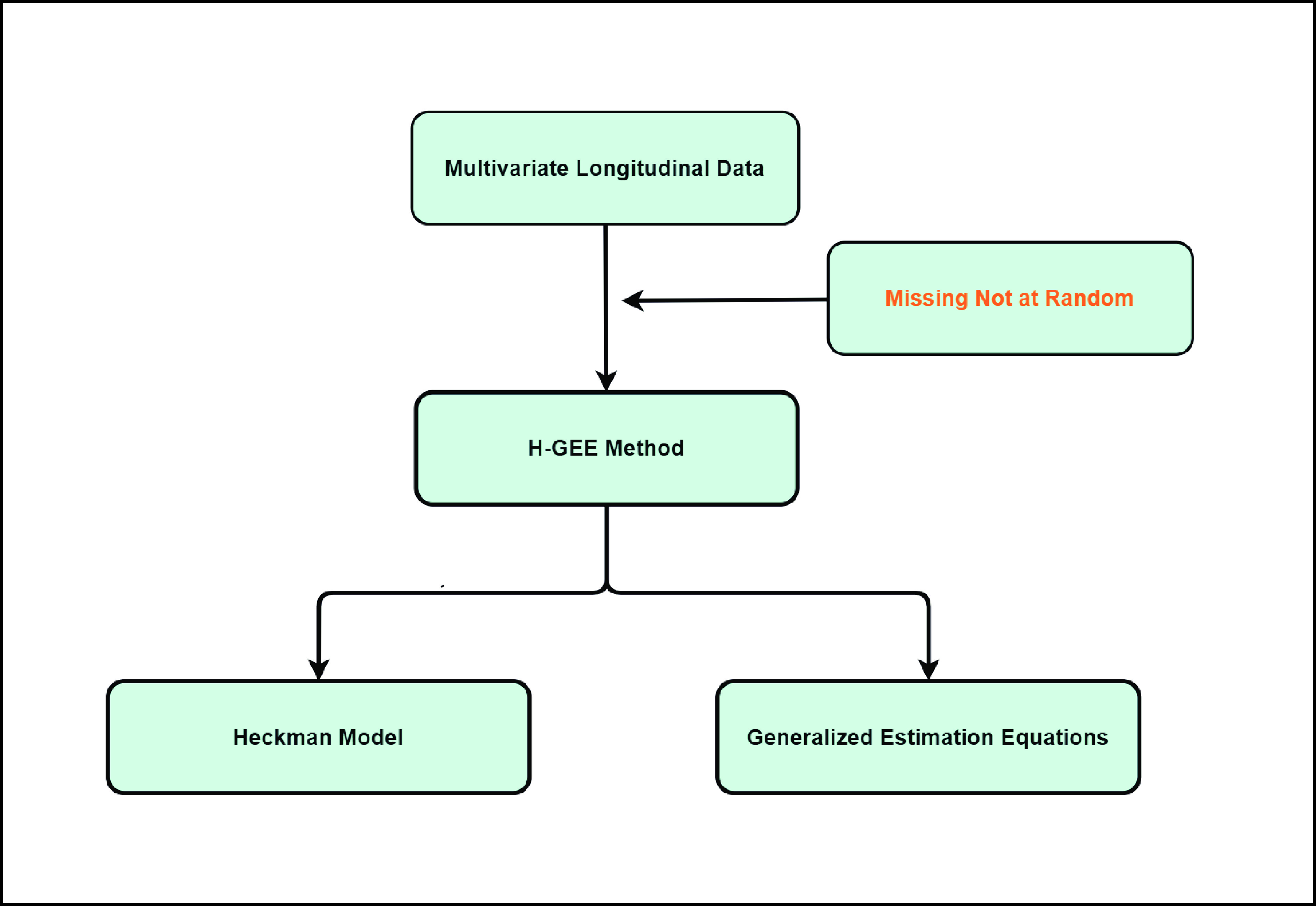
Graphical Abstract
H-GEE method flowchart.
Abstract
In the interdisciplinary realm of statistics, genetics, and epidemiology, longitudinal sibling pair data offers a unique perspective for investigating complex diseases and traits, allowing the exploration of the dynamic processes of gene expression over time by controlling numerous confounding factors. Missing-not-at-random (MNAR) data are commonly used in such types of studies, but no statistical methods specifically tailored have been developed to handle MNAR data in complex longitudinal data in the literature. Here, we propose a new statistical method by jointly modeling longitudinal data from sib-pairs and MNAR data. Extensive simulations demonstrate the excellent finite sample properties of the proposed method.
Public Summary
The challenge in longitudinal studies lies in effectively addressing missing-not-at-random (MNAR) data, which complicates data analysis.
The proposed H-GEE method, combining the Heckman model and generalized estimating equations (GEE), aims to overcome MNAR challenges for robust data analysis.
Extensive simulations validate H-GEE’s effectiveness in handling MNAR data, highlighting its potential for advancing genetic and epidemiological research.
Longitudinal sibling pair data refers to genetic and phenotypic data collected from siblings within a family over time by controlling numerous confounding factors. This type of data is widely applied in fields such as genetic epidemiology and behavioral genetics, which can capture the changes in phenotype states and their genetic and environmental influences over time. Researchers leverage such data, especially those collected at multiple time points, to track phenotypic trajectories, uncover potential patterns or trends, and assess differences in responses to specific events or interventions among siblings. This study design proves particularly effective in exploring genes related to complex phenotypes such as hypertension, diabetes, heart disease, and height, as it allows researchers to control for many difficult-to-measure potential confounding factors, such as family background and other environmental influences[1].
In summary, longitudinal sibling pair data provides a unique perspective for exploring the genetic and environmental factors underlying complex phenotypes. For instance, Friedlander et al.[2] proposed a method to adjust covariates in longitudinal sibling pair data and applied it to blood pressure data from the Framingham Heart Study. Guo et al.[3] employed stepwise discriminant analysis techniques to analyze chromosome data from the Framingham Heart Study, revealing interactions between genes and genes, as well as genes and the environment related to hypertension. Additionally, Keyes et al.[4] analyzed twin data to study the developmental trajectories of illicit drug use, while Silventoinen et al.[5] used twin data from multiple countries to investigate the heritability of adult height. These studies underscore the importance of longitudinal sibling pair data in exploring how genetic and environmental factors collectively influence phenotypic development.
However, collecting such data poses challenges, with the most common issue being data missingness, especially non-random missingness. Discarding such data may result in information loss and distorted inference results. Therefore, specialized statistical methods are necessary for the analysis of longitudinal sibling pair data to elucidate the correlation between siblings, make full use of the observed information, and achieve reliable statistical inferences. Despite these challenges, longitudinal sibling pair data is crucial for understanding the genetic and environmental factors involved in the development of complex diseases and traits, providing a theoretical foundation for future personalized therapies and intervention strategies.
Most existing methods focus on the analysis of complete longitudinal sibling data, neglecting the issue of missing data. For complete longitudinal sibling data, methods for handling longitudinal data can be utilized, taking into account the dependency between siblings. There is extensive literature on the analysis of univariate longitudinal data[6–9]. Everitt and Dunn[10] provided a brief yet systematic method for analyzing continuous and categorical responses to longitudinal measurements. Dunlop[11] offered a clear description of regression methods for longitudinal data. Laird et al.[12] described formulas for longitudinal data random-effects models. Detailed discussions on maximum likelihood estimation methods based on the expectation-maximization (EM) algorithm were provided by Laird et al.[13] and others. Liang and Zeger[14] discussed the use of generalized estimating equations (GEE).
There is limited research in the existing literature regarding the study of longitudinal sibling data with missing data. Missing data mechanisms are generally categorized as missing completely at random (MCAR), missing at random (MAR), and missing not at random (MNAR)[15]. For managing MCAR and MAR data, interpolation methods were commonly employed, as discussed in the works of Little et al.[16] and Sterne et al[17]. Notably, Schafer and Graham[18] along with Graham[19] provided comprehensive descriptions of various existing methods. In this paper, we focus on MNAR data and propose a two-step method. In the first step, we estimate missing data based on the Heckman model[20]. In the second step, we propose to use generalized estimation equations to estimate unknown parameters. A bootstrap strategy is adopted to deal with the variability due to the estimated missing data. The validity of our proposed method was confirmed through extensive simulations.
2.
Method
2.1
Notations and models
Let Yijk represent the continuous phenotype of the j-th sibling in the i-th family at time point tijk (k=1⋯,nij). This paper focuses on the association between phenotypes and genetic markers (single nucleotide polymorphisms, SNPs). Subsequently, the term “test locus” is used to refer to such genetic markers. Let A and a denote the major and minor alleles of the test locus, respectively. Let Xij represent the genotype of the j-th sibling in the i-th family (0 for AA, 1 for Aa, and 2 for aa).
We use the following linear model to characterize the influence of genotypes on phenotypes (outcome model):
Yijk=α+βXXij+βttijk+γXijtijk+ηi+ηij+ηktijk+εijk.
(1)
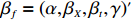
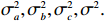
Here, βf=(α,βX,βt,γ)′ is a fixed effect vector; ηi, ηij, and ηijk are independent normally distributed random effects with mean zero and variances σ2a, σ2b, and σ2c, respectively; εijk is the random error following the normal distribution with mean 0 and variance σ2. Note that the three random effects reflect variability due to family, individual, and time.
The MNAR mechanism of the phenotype is modeled through the following Heckman model (selection model) [20]:
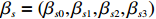
where z⋆ijk is an underlying continuous variable and z⋆ijk is the missingness indicator (zijk=1 if Yijk is observed and zijk=0 if Yijk is missing); I is the indicator function (I(A)=1 if A occurs and I(A)=0 otherwise); uijk is the error term following the standard normal distribution; βs=(βs0,βs1,βs2,βs3) is a vector of fixed effects.
The joint model comprises the outcome model (1) and the selection model (2). Let ρ denote the correlation coefficient between uijk and εijk. Let Y⋆ijk denote the observed outcome (Y⋆ijk=Yijkzijk), then all observed data are (Y∗ijk,tijk,Xij,zijk), i=1,⋯,n;j=1,2;k=1,⋯,nij. All unknown parameters are βs, βf, σ2a,σ2b,σ2c,σ2.
The joint model (1)-(2) extends the Heckman model from several aspects. First, the phenotype model utilizes three random effects to characterize variability at the levels of family, individual, and time. Second, the joint model does not require εijk to be normaly distributed. These two distinctions significantly broaden the applicability of the Heckman model. In the following subsection, we propose to use a generalized estimating equation (GEE) to accommodate the non-normal distribution assumption.
2.2
A two-step estimation method
If follows from (1)-(2) that the conditional expectation of the observed outcome is
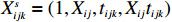
Xsijk=(1,Xij,tijk,Xijtijk), ϕ is the probability density function of the normal distribution, and Φ is the cumulative distribution function of the standard normal distribution.
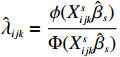
We employ a two-step method to separately estimate the parameter vectors βs and βf. In the first step, we can estimate βs by the maximum likelihood estimator, denoted by ˆβs, based on the selection model (2). In the second step, we first replace λijk by ˆλijk=ϕ(Xsijkˆβs)Φ(Xsijkˆβs), yielding the linear model
Y⋆ijk=α+βXXij+βttijk+γXijtijk+ρσˆλijk+eijk,
where eijk is a random error with mean 0. Then, we employ the GEE method to estimate βf and ρσ. This two-step method does not need to specify the distributional form of Yijk, thus it is robust to a certain degree. In what follows, we provide the detailed parameter estimation procedure and discuss the corresponding asymptotic properties.
The first step of the estimation algorithm is to estimate the parameter vector βs by the maximum likelihood method, which is based on the log-likelihood function for the observed data (zijk,Xij,tijk), i=1,⋯,n;j=1,2;k=1,⋯,nij:
where ΣYi is a working covariance matrix of Yi. In practice, we can specify the correlation matrix Ri(ξ) of Yi, leading to the working covariance matrix
˜ΣYi=σ2Ri(ξ).
Some commonly used correlation coefficient structures include independence structure, exchangeable correlation structure, one-dependent structure, autocorrelation, and unstructured correlation. Regardless of the choice of correlation coefficient structure, under suitable regularity conditions (eg., the variance of Yijk, denoted by σ2, is independent of i, j, and k), the corresponding GEE estimator ˆβ is consistent for β and asymptotically normal:
√n(ˆβ−β)→N(0,Gβ), with Gβ=σ2[E{1n∂S(β)∂β′}]−1.
Estimates of β and Gβ can be obtained by applying the existing GEE procedures implemented existing programs. Note that in model (3), ˆλijk shares a common random variable ˆβ, resulting in correlation between Y⋆ijk. While the existing standard GEE procedures can produce consistent parameter estimates, they may underestimate the covariance matrix Gβ due to the correlation between Y⋆ijk. To address this issue, we propose to adopt the bootstrap method, which can provide a consistent estimate of Gβ.
3.
A simulation study
We conducted a simulation study to evaluate the performance of our Heckman-model-based method, referred to as H-GEE. We also considered two additional methods C-GLM and D-GLM. C-GLM directly fitted the generalized linear model to complete data. On the other hand, D-GLM fitted the generalized linear model to the observed data by discarding missing data. Both C-GLM and D-GLM were implemented by the R function lmer in the R package lme4. The R functions nlminb and lmer were adopted to in the first step and the second step of H-GEE, respectively. It is noteworthy that C-GLM is not applicable in practical scenarios since it assumes that missing data are observable. C-GLM was simply used as a gold standard method.
The simulated data were generated as follows. First, under the assumption of Hardy-Weinberg equilibrium, genotypes of a single nucleotide polymorphism with minor allele frequency 0.25 were independently generated for 100N individuals. Genetypes of N couples were then drawn from these genotypes by assuming random mating. Genotypes (Xi1,Xi2) of two offspring were generated for each of N couples based on Mendel’s laws of inheritance. Then, set the model parameters βf, σ2a, σ2b, σ2c, βs, ρ, and σ2 in models (1)-(2), such that the proportion of error variance to total variance was approximately 80% by setting σ2=2(β20+β21+γ2+σ2a+σ2b+σ2c). Next, the age tijk was randomly drawn from the uniform distribution U(45,75). Finally, Yijk and z⋆ijk were generated according to models (1)-(2). The number of time points, k, followed the uniform distribution in {2,4,5}: P(k=3)=P(k=4)=P(k=5)=1/3. The parameters were fixed as σ2a=0.5, σ2b=0.25, σ2c=0.05, βs=(βs0,1,1,1), ρ=0.75, and βf=(5,2,1,0).
In all simulations, the default sample size, interaction effect, and missing rate were fixed at n=100, γ=0, and 0.2 (corresponding to βs0=1.5), unless specified otherwise. We examined the performance of the considered methods under various effect sizes, sample sizes, missing rates, and error distributions. We also evaluated the validity of the bootstrap method for estimating the standard errors of parameter estimates.
First, we examined the estimation and test results of various genotype-time interaction effects for the three considered methods. We considered four different values of interaction effects (γ=0, 0.25, 0.5, and 1). The sample size was fixed at n=100. The simulation results based on 500 replicates are presented in Table 1. Both C-GLM and H-GEE produced very virtually unbiased estimates for the fixed effects βf, while D-GLM had considerable estimation biases, especially when γ was large. These results demonstrated that simply deleting incomplete data could lead to very biased estimation results in the presence of MNAR data, while the proposed method H-GEE could effectively adjust such biases. Due to missing data, H-GEE was less efficient than C-GLM. For example, the standard errors of the γ estimates by H-GEE were around 1.2 times those of C-GLM. The estimated standard errors of H-GEE were considerably smaller than the empirical ones (results not shown), indicating the necessity of employing the bootstrap method. The performance of the bootstrap method will be examined at the end of this section.
Table
1.
Estimation biases (standard errors) with various interaction effects.
γa
Methodb
ˆα0c
ˆβ0d
ˆβ1e
ˆγ
^ρσf
0.00
C-GLM
0.00 (0.17)
0.00 (0.16)
−0.01 (0.16)
−0.00 (0.17)
−
D-GLM
1.15 (0.18)
−0.39 (0.18)
−0.56 (0.17)
−0.25 (0.19)
−
H-GEE
0.02 (0.46)
−0.00 (0.22)
−0.02 (0.27)
−0.00 (0.21)
−0.04 (1.31)
0.25
C-GLM
0.00 (0.17)
0.00 (0.16)
−0.01 (0.16)
0.00 (0.17)
−
D-GLM
1.15 (0.18)
−0.39 (0.18)
−0.56 (0.18)
−0.25 (0.19)
−
H-GEE
0.02 (0.46)
0.00 (0.22)
−0.02 (0.27)
0.00 (0.21)
−0.03 (1.32)
0.50
C-GLM
0.00 (0.17)
0.00 (0.16)
−0.01 (0.16)
0.00 (0.17)
−
D-GLM
1.17 (0.18)
−0.40 (0.18)
−0.57 (0.18)
−0.25 (0.20)
−
H-GEE
0.02 (0.47)
0.00 (0.23)
−0.02 (0.27)
0.00 (0.21)
0.03 (1.33)
1.00
C-GLM
0.00 (0.18)
0.00 (0.17)
−0.01 (0.17)
0.00 (0.18)
−
D-GLM
1.24 (0.19)
−0.42 (0.19)
−0.60 (0.19)
−0.27 (0.21)
−
H-GEE
0.02 (0.50)
0.00 (0.24)
−0.02 (0.29)
0.00 (0.22)
0.25 (1.41)
aThe true value of γ. bC-GLM, the method fitting GLM with complete data; D-GLM, the method fitting GLM dropping incomplete data; H-GEE, the proposed method based on the Heckman model. cThe true value of α0 was 5. dThe true value of β0 was 2. eThe true value of β1 was 1. fThe true value ρσ was 3.554.
Second, we evaluated the performance of the considered methods under different sample sizes (n= 50, 100, 200, 300, and 400). As shown in Table 2, both C-GLM and H-GEE were virtually unbiased under various sample sizes. As expected, the standard errors (SE) decreased when the sample size increased. The estimation bias of D-GLM tended to be stable with the increasing sample size, indicating systematic estimation biases of D-GLM.
Table
2.
Estimation biases (standard errors) with different sample sizes.
Na
Methodb
ˆα0c
ˆβ0d
ˆβ1e
ˆγf
^ρσg
50
C-GLM
−0.01 (0.23)
0.01 (0.23)
0.00 (0.23)
−0.01 (0.22)
−
D-GLM
1.13 (0.24)
−0.40 (0.26)
−0.55 (0.26)
−0.25 (0.28)
−
H-GEE
0.04 (0.59)
−0.01 (0.36)
−0.03 (0.30)
−0.02 (1.66)
−0.16 (0.32)
100
C-GLM
0.00 (0.17)
0.00 (0.16)
−0.01 (0.16)
0.00 (0.17)
−
D-GLM
5.15 (0.18)
−0.39 (0.18)
−0.56 (0.17)
−0.25 (0.19)
−
H-GEE
0.02 (0.46)
0.00 (0.22)
−0.02 (0.27)
0.00 (0.21)
−0.05 (1.31)
200
C-GLM
0.00 (0.12)
0.00 (0.11)
0.01 (0.12)
0.00 (0.11)
−
D-GLM
5.14 (0.12)
−0.38 (0.13)
−0.54 (0.12)
−0.24 (0.14)
−
H-GEE
0.02 (0.33)
0.00 (0.16)
0.00 (0.19)
0.00 (0.14)
−0.04 (0.91)
300
C-GLM
0.00 (0.09)
0.00 (0.10)
−0.01 (0.10)
0.00 (0.09)
−
D-GLM
1.15 (0.10)
−0.37 (0.11)
−0.56 (0.10)
−0.24 (0.11)
−
H-GEE
0.01 (0.24)
0.00 (0.12)
−0.01 (0.15)
0.00 (0.12)
−0.01 (0.67)
400
C-GLM
0.00 (0.08)
−0.01 (0.08)
0.00 (0.08)
0.00 (0.08)
−
D-GLM
1.15 (0.09)
−0.39 (0.09)
−0.55 (0.09)
−0.25 (0.10)
−
H-GEE
0.01 (0.23)
−0.01 (0.11)
0.00 (0.14)
0.00 (0.11)
−0.03 (0.64)
aThe number of families. bC-GLM, the method fitting GLM with complete data; D-GLM, the method fitting GLM dropping incomplete data; H-GEE, the proposed method based on the Heckman model. cThe true value of α0 was 5. dThe true value of β0 was 2. eThe true value of β1 was 1. fThe true value of γ was 0. gThe true value of ρσ was 3.554.
Third, we examined the performance of the considered methods under different missing rates (0.05, 0.1, 0.2, 0.3, and 0.6), with the corresponding values of βs0 being 3, 2, 1.5, 0, and –1.5, respectively. As shown in Table 3, the estimation bias of D-GLM dramatically increased as the missing rate increased, while the estimation bias of H-GEE remained to be very minor.
Table
3.
Estimation biases (standard errors) with different missing rates.
Ratea
Methodb
ˆα0c
ˆβ0d
ˆβ1e
ˆγf
^ρσg
0.05
C-GLM
0.00 (0.17)
0.00 (0.16)
−0.01 (0.16)
0.00 (0.17)
−
D-GLM
0.32 (0.17)
−0.03 (0.16)
−0.24 (0.16)
−0.14 (0.17)
−
H-GEE
0.02 (0.26)
0.00 (0.16)
−0.02 (0.22)
−0.01 (0.20)
−0.09 (2.26)
0.10
C-GLM
0.00 (0.17)
0.00 (0.16)
−0.01 (0.16)
0.00(0.17)
−
D-GLM
0.66 (0.17)
−0.16 (0.17)
−0.40 (0.17)
−0.20 (0.18)
−
H-GEE
0.02 (0.34)
0.00 (0.18)
−0.02 (0.24)
−0.01 (0.20)
−0.05 (1.61)
0.20
C-GLM
0.00 (0.17)
0.00 (0.16)
−0.01 (0.16)
0.00 (0.17)
−
D-GLM
5.15 (0.18)
−0.39 (0.18)
−0.56 (0.17)
−0.25 (0.19)
−
H-GEE
0.02 (0.46)
0.00 (0.22)
−0.02 (0.27)
0.00 (0.21)
−0.05 (1.31)
0.30
C-GLM
0.00 (0.17)
0.00 (0.16)
−0.01 (0.16)
0.00 (0.17)
−
D-GLM
1.61 (0.18)
−0.61 (0.18)
−0.68 (0.18)
−0.29 (0.21)
−
H-GEE
0.02 (0.56)
0.00 (0.27)
−0.02 (0.28)
0.00(0.22)
−0.03 (1.14)
0.60
C-GLM
0.00 (0.17)
0.00 (0.16)
−0.01 (0.16)
0.00 (0.17)
−
D-GLM
3.40 (0.25)
−1.41 (0.25)
−1.14 (0.28)
−0.42 (0.33)
−
H-GEE
0.02 (0.90)
0.00 (0.43)
−0.02 (0.38)
0.00 (0.30)
−0.03 (0.87)
aThe proportion of missing data. bC-GLM, the method fitting GLM with complete data; D-GLM, the method fitting GLM dropping incomplete data; H-GEE, the proposed method based on the Heckman model. cThe true value of α0 was 5. dThe true value of β0 was 2. eThe true value of β1 was 1. fThe true value of γ was 0. gThe true value of ρσ was 3.555.
Fourth, we examined the performance of the considered methods under several typical non-normal error distributions. Two non-normal distributions were considered: the t-distribution with 5 degrees of freedom and the skewed normal distribution with skewness parameter 5. As shown in Table 4, C-GLM and H-GEE were again virtually unbiased, while D-GLM had systematic estimation biases.
Table
4.
Estimation biases (standard errors) with different error distributions.
Errora
Methodb
ˆα0c
ˆβ0d
ˆβ1e
ˆγf
^ρσg
N(0,1)
C-GLM
0.00 (0.17)
0.00 (0.16)
−0.01 (0.16)
0.00 (0.17)
−
D-GLM
1.15 (0.18)
−0.39 (0.18)
−0.56 (0.17)
−0.25 (0.19)
−
H-GEE
0.02 (0.46)
0.00 (0.22)
−0.02 (0.27)
0.00 (0.21)
−0.05 (1.31)
t5
C-GLM
0.00 (0.10)
0.01 (0.09)
0.00 (0.09)
0.00 (0.09)
−
D-GLM
0.49 (0.10)
−0.15 (0.10)
−0.23 (0.10)
−0.11 (0.10)
−
H-GEE
0.01 (0.25)
0.01 (0.12)
0.00 (0.15)
0.00 (0.12)
−2.07 (0.69)
SN(5)
C-GLM
0.01 (0.09)
0.00 (0.07)
0.00 (0.06)
0.00 (0.06)
−
D-GLM
0.01 (0.09)
0.00 (0.08)
−0.01 (0.07)
0.00 (0.07)
−
H-GEE
0.02 (0.20)
0.00 (0.10)
−0.02 (0.11)
0.00 (0.09)
−3.61 (0.56)
aThe error distribution: N(0,1), the standard normal distribution; t5, the t-distribution with 5 degrees of freedom; SN(5), the skewed normal distribution with the location parameter of 5. bC-GLM, the method fitting GLM with complete data; D-GLM, the method fitting GLM dropping incomplete data; H-GEE, the proposed method based on the Heckman model. cThe true value of α0 was 5. dThe true value of β0 was 2. eThe true value of β1 was 1. fThe true value of γ was 0. gThe true value of ρσ was 3.555.
Finally, we examined the bootstrap method for estimating standard errors in H-GEE. Let the version of H-GEE incorporating the bootstrap method be denoted by H-GEE-B. The simulation results corresponding to Table 1 are presented in Table 5. Evidently, the estimated standard errors were close to the empirical ones for all parameters, and the corresponding coverage probabilities were close to the nominal level 0.95. This demonstrated the validity of the bootstrap method.
Table
5.
Simulation results using the bootstrap method.
γa
ˆα0
ˆβ0
ˆβ1
ˆγ
SEb
SEEc
CPd
SE
SEE
Bias
SE
SEE
CP
SE
SEE
CP
0.00
0.45
0.45
0.93
0.23
0.22
0.94
0.26
0.27
0.95
0.21
0.21
0.94
0.25
0.46
0.45
0.93
0.23
0.22
0.94
0.26
0.27
0.95
0.21
0.21
0.93
0.50
0.46
0.46
0.93
0.23
0.23
0.94
0.27
0.28
0.95
0.21
0.21
0.93
1.00
0.48
0.47
0.93
0.24
0.23
0.94
0.27
0.28
0.95
0.22
0.22
0.94
aTrue value of γ; bempirical standard error; cmean estimated standard error; dcoverage probability of 95% confidence interval.
With the progress of bioinformatics and epidemiology, the understanding of complex diseases and traits continues to deepen. The longitudinal sibling pair data provides researchers with the opportunity to explore in detail the patterns of genetic changes over time, offering a crucial means for interpreting the connection between genes and complex diseases and traits. Its profound value lies in its ability to help researchers delve into the interaction between genes and time, bringing new research directions to the fields of genetics and epidemiology.
To further explore this dynamic relationship, this study adopts a longitudinal research strategy and collects sibling pair data at multiple time points. However, this research strategy comes with challenges, such as MNAR outcomes. There is a lack of literature on methods for handling MNAR outcomes in longitudinal studies. To address this issue, this paper proposes a novel method H-GEE, which combines the Heckman model and generalized estimating equations (GEE). H-GEE enables effective statistical analysis of longitudinal sibling pair data in the presence of MNAR outcomes. Extensive simulation studies confirmed the feasibility of this method under limited samples. H-GEE exhibited a reasonably good performance in our simulation studies.
H-GEE has its limitations. Currently, it can only handle continuous response variables, and it deserves to be extended to other types of response variables such as binary response variables, count response variables, and survival time response variables. Additionally, although the bootstrap method is valid in estimating standard errors, it is time consuming. It deserves further investigation to derive the asymptotic distribution of estimators, so that an explicit standard error estimator can be obtained.
Acknowledgements
The authors thank the students in Prof. Hong Zhang’s laboratory for their support. This work was supported by the National Natural Science Foundation of China (12171451).
Conflict of interest
The authors declare that they have no conflict of interest.
The challenge in longitudinal studies lies in effectively addressing missing-not-at-random (MNAR) data, which complicates data analysis.
The proposed H-GEE method, combining the Heckman model and generalized estimating equations (GEE), aims to overcome MNAR challenges for robust data analysis.
Extensive simulations validate H-GEE’s effectiveness in handling MNAR data, highlighting its potential for advancing genetic and epidemiological research.
Rutter M. Nature, nurture, and development: From evangelism through science toward policy and practice. Child Development, 2002, 73 (1): 1–21. DOI: 10.1111/1467-8624.00388
[2]
Friedlander Y, Talmud P J, Edwards K L, et al. Sib-pair linkage analysis of longitudinal changes in lipoprotein risk factors and lipase genes in women twins. Journal of Lipid Research, 2000, 41 (8): 1302–1309. DOI: 10.1016/S0022-2275(20)33438-6
[3]
Guo Z, Li X, Rao S Q, et al. Multivariate sib-pair linkage analysis of longitudinal phenotypes by three step-wise analysis approaches. BMC Genetics, 2003, 4 (1): 1–7. DOI: 10.1186/1471-2156-4-1
[4]
Keyes M A, Malone S M, Elkins I J, et al. The enrichment study of the Minnesota twin family study: increasing the yield of twin families at high risk for externalizing psychopathology. Twin Research and Human Genetics, 2009, 12 (5): 489–501. DOI: 10.1375/twin.12.5.489
[5]
Silventoinen K, Sammalisto S, Perola M, et al. Heritability of adult body height: A comparative study of twin cohorts in eight countries. Twin Research, 2003, 6 (5): 399–408. DOI: 10.1375/136905203770326402
[6]
Hand D M, Crowder M J. Practical Longitudinal Data Analysis. New York: Chapman & Hall/CRC, 1996 .
[7]
Verbeke G. Linear mixed models for longitudinal data. In: Linear Mixed Models in Practice. New York: Springer, 1997 .
[8]
Diggle P, Heagerty P, Liang K Y, et al. Analysis of Longitudinal Data. New York: Oxford University Press, 2002 .
[9]
Fitzmaurice G M, Laird N M, Ware J H. Applied Longitudinal Analysis. Hoboken, USA: Wiley, 2012 .
[10]
Everitt B S, Dunn G. Applied Multivariate Data Analysis. Second Edition. Chichester, UK: Wiley, 2001 .
[11]
Dunlop D D. Regression for longitudinal data: a bridge from least squares regression. The American Statistician, 1994, 48 (4): 299–303. DOI: 10.1080/00031305.1994.10476085
[12]
Laird N M, Ware J H. Random-effects models for longitudinal data. Biometrics, 1982, 38 (4): 963–974. DOI: 10.2307/2529876
[13]
Laird N M, Lange N, Stram D. Maximum likelihood computations with repeated measures: application of the EM algorithm. Journal of the American Statistical Association, 1987, 82 (397): 97–105. DOI: 10.1080/01621459.1987.10478395
[14]
Liang K Y, Zeger S L. Longitudinal data analysis using generalized linear models. Biometrika, 1986, 73 (1): 13–22. DOI: 10.1093/biomet/73.1.13
[15]
Little R J, Rubin D B. Statistical Analysis with Missing Data. Third Edition. Hoboken, USA: Wiley, 2019 .
[16]
Little R J. Pattern-mixture models for multivariate incomplete data. Journal of the American Statistical Association, 1993, 88 (421): 125–134. DOI: 10.1080/01621459.1993.10594302
[17]
Sterne J A, Carlin J B, Royston P, et al. Multiple imputation for missing data in epidemiological and clinical research: potential and pitfalls. BMJ, 2009, 338: b2393. DOI: 10.1136/bmj.b2393
[18]
Schafer J L, Graham J W. Missing data: Our view of the state of the art. Psychological Methods, 2002, 7 (2): 147–177. DOI: 10.1037/1082-989X.7.2.147
[19]
Graham J W. Missing data analysis: Making it work in the real world. Annual Review of Psychology, 2009, 60: 549–576. DOI: 10.1146/annurev.psych.58.110405.085530
[20]
Heckman J J. Sample selection bias as a specification error. The Econometric Society, 1979, 47 (1): 153–161. DOI: 10.2307/1912352
Table
1.
Estimation biases (standard errors) with various interaction effects.
γa
Methodb
ˆα0c
ˆβ0d
ˆβ1e
ˆγ
^ρσf
0.00
C-GLM
0.00 (0.17)
0.00 (0.16)
−0.01 (0.16)
−0.00 (0.17)
−
D-GLM
1.15 (0.18)
−0.39 (0.18)
−0.56 (0.17)
−0.25 (0.19)
−
H-GEE
0.02 (0.46)
−0.00 (0.22)
−0.02 (0.27)
−0.00 (0.21)
−0.04 (1.31)
0.25
C-GLM
0.00 (0.17)
0.00 (0.16)
−0.01 (0.16)
0.00 (0.17)
−
D-GLM
1.15 (0.18)
−0.39 (0.18)
−0.56 (0.18)
−0.25 (0.19)
−
H-GEE
0.02 (0.46)
0.00 (0.22)
−0.02 (0.27)
0.00 (0.21)
−0.03 (1.32)
0.50
C-GLM
0.00 (0.17)
0.00 (0.16)
−0.01 (0.16)
0.00 (0.17)
−
D-GLM
1.17 (0.18)
−0.40 (0.18)
−0.57 (0.18)
−0.25 (0.20)
−
H-GEE
0.02 (0.47)
0.00 (0.23)
−0.02 (0.27)
0.00 (0.21)
0.03 (1.33)
1.00
C-GLM
0.00 (0.18)
0.00 (0.17)
−0.01 (0.17)
0.00 (0.18)
−
D-GLM
1.24 (0.19)
−0.42 (0.19)
−0.60 (0.19)
−0.27 (0.21)
−
H-GEE
0.02 (0.50)
0.00 (0.24)
−0.02 (0.29)
0.00 (0.22)
0.25 (1.41)
aThe true value of γ. bC-GLM, the method fitting GLM with complete data; D-GLM, the method fitting GLM dropping incomplete data; H-GEE, the proposed method based on the Heckman model. cThe true value of α0 was 5. dThe true value of β0 was 2. eThe true value of β1 was 1. fThe true value ρσ was 3.554.
Table
2.
Estimation biases (standard errors) with different sample sizes.
Na
Methodb
ˆα0c
ˆβ0d
ˆβ1e
ˆγf
^ρσg
50
C-GLM
−0.01 (0.23)
0.01 (0.23)
0.00 (0.23)
−0.01 (0.22)
−
D-GLM
1.13 (0.24)
−0.40 (0.26)
−0.55 (0.26)
−0.25 (0.28)
−
H-GEE
0.04 (0.59)
−0.01 (0.36)
−0.03 (0.30)
−0.02 (1.66)
−0.16 (0.32)
100
C-GLM
0.00 (0.17)
0.00 (0.16)
−0.01 (0.16)
0.00 (0.17)
−
D-GLM
5.15 (0.18)
−0.39 (0.18)
−0.56 (0.17)
−0.25 (0.19)
−
H-GEE
0.02 (0.46)
0.00 (0.22)
−0.02 (0.27)
0.00 (0.21)
−0.05 (1.31)
200
C-GLM
0.00 (0.12)
0.00 (0.11)
0.01 (0.12)
0.00 (0.11)
−
D-GLM
5.14 (0.12)
−0.38 (0.13)
−0.54 (0.12)
−0.24 (0.14)
−
H-GEE
0.02 (0.33)
0.00 (0.16)
0.00 (0.19)
0.00 (0.14)
−0.04 (0.91)
300
C-GLM
0.00 (0.09)
0.00 (0.10)
−0.01 (0.10)
0.00 (0.09)
−
D-GLM
1.15 (0.10)
−0.37 (0.11)
−0.56 (0.10)
−0.24 (0.11)
−
H-GEE
0.01 (0.24)
0.00 (0.12)
−0.01 (0.15)
0.00 (0.12)
−0.01 (0.67)
400
C-GLM
0.00 (0.08)
−0.01 (0.08)
0.00 (0.08)
0.00 (0.08)
−
D-GLM
1.15 (0.09)
−0.39 (0.09)
−0.55 (0.09)
−0.25 (0.10)
−
H-GEE
0.01 (0.23)
−0.01 (0.11)
0.00 (0.14)
0.00 (0.11)
−0.03 (0.64)
aThe number of families. bC-GLM, the method fitting GLM with complete data; D-GLM, the method fitting GLM dropping incomplete data; H-GEE, the proposed method based on the Heckman model. cThe true value of α0 was 5. dThe true value of β0 was 2. eThe true value of β1 was 1. fThe true value of γ was 0. gThe true value of ρσ was 3.554.
Table
3.
Estimation biases (standard errors) with different missing rates.
Ratea
Methodb
ˆα0c
ˆβ0d
ˆβ1e
ˆγf
^ρσg
0.05
C-GLM
0.00 (0.17)
0.00 (0.16)
−0.01 (0.16)
0.00 (0.17)
−
D-GLM
0.32 (0.17)
−0.03 (0.16)
−0.24 (0.16)
−0.14 (0.17)
−
H-GEE
0.02 (0.26)
0.00 (0.16)
−0.02 (0.22)
−0.01 (0.20)
−0.09 (2.26)
0.10
C-GLM
0.00 (0.17)
0.00 (0.16)
−0.01 (0.16)
0.00(0.17)
−
D-GLM
0.66 (0.17)
−0.16 (0.17)
−0.40 (0.17)
−0.20 (0.18)
−
H-GEE
0.02 (0.34)
0.00 (0.18)
−0.02 (0.24)
−0.01 (0.20)
−0.05 (1.61)
0.20
C-GLM
0.00 (0.17)
0.00 (0.16)
−0.01 (0.16)
0.00 (0.17)
−
D-GLM
5.15 (0.18)
−0.39 (0.18)
−0.56 (0.17)
−0.25 (0.19)
−
H-GEE
0.02 (0.46)
0.00 (0.22)
−0.02 (0.27)
0.00 (0.21)
−0.05 (1.31)
0.30
C-GLM
0.00 (0.17)
0.00 (0.16)
−0.01 (0.16)
0.00 (0.17)
−
D-GLM
1.61 (0.18)
−0.61 (0.18)
−0.68 (0.18)
−0.29 (0.21)
−
H-GEE
0.02 (0.56)
0.00 (0.27)
−0.02 (0.28)
0.00(0.22)
−0.03 (1.14)
0.60
C-GLM
0.00 (0.17)
0.00 (0.16)
−0.01 (0.16)
0.00 (0.17)
−
D-GLM
3.40 (0.25)
−1.41 (0.25)
−1.14 (0.28)
−0.42 (0.33)
−
H-GEE
0.02 (0.90)
0.00 (0.43)
−0.02 (0.38)
0.00 (0.30)
−0.03 (0.87)
aThe proportion of missing data. bC-GLM, the method fitting GLM with complete data; D-GLM, the method fitting GLM dropping incomplete data; H-GEE, the proposed method based on the Heckman model. cThe true value of α0 was 5. dThe true value of β0 was 2. eThe true value of β1 was 1. fThe true value of γ was 0. gThe true value of ρσ was 3.555.
Table
4.
Estimation biases (standard errors) with different error distributions.
Errora
Methodb
ˆα0c
ˆβ0d
ˆβ1e
ˆγf
^ρσg
N(0,1)
C-GLM
0.00 (0.17)
0.00 (0.16)
−0.01 (0.16)
0.00 (0.17)
−
D-GLM
1.15 (0.18)
−0.39 (0.18)
−0.56 (0.17)
−0.25 (0.19)
−
H-GEE
0.02 (0.46)
0.00 (0.22)
−0.02 (0.27)
0.00 (0.21)
−0.05 (1.31)
t5
C-GLM
0.00 (0.10)
0.01 (0.09)
0.00 (0.09)
0.00 (0.09)
−
D-GLM
0.49 (0.10)
−0.15 (0.10)
−0.23 (0.10)
−0.11 (0.10)
−
H-GEE
0.01 (0.25)
0.01 (0.12)
0.00 (0.15)
0.00 (0.12)
−2.07 (0.69)
SN(5)
C-GLM
0.01 (0.09)
0.00 (0.07)
0.00 (0.06)
0.00 (0.06)
−
D-GLM
0.01 (0.09)
0.00 (0.08)
−0.01 (0.07)
0.00 (0.07)
−
H-GEE
0.02 (0.20)
0.00 (0.10)
−0.02 (0.11)
0.00 (0.09)
−3.61 (0.56)
aThe error distribution: N(0,1), the standard normal distribution; t5, the t-distribution with 5 degrees of freedom; SN(5), the skewed normal distribution with the location parameter of 5. bC-GLM, the method fitting GLM with complete data; D-GLM, the method fitting GLM dropping incomplete data; H-GEE, the proposed method based on the Heckman model. cThe true value of α0 was 5. dThe true value of β0 was 2. eThe true value of β1 was 1. fThe true value of γ was 0. gThe true value of ρσ was 3.555.


 DownLoad:


